mixLin = {
  const mat = (v1, v2, rho) => {
    const s1 = Math.sqrt(v1), s2 = Math.sqrt(v2);
    return [[v1, rho * s1 * s2], [rho * s1 * s2, v2]];
  };
  const add = (A, B, x, y) => [
    [x * A[0][0] + y * B[0][0], x * A[0][1] + y * B[0][1]],
    [x * A[1][0] + y * B[1][0], x * A[1][1] + y * B[1][1]]
  ];
  const det = (S) => S[0][0] * S[1][1] - S[0][1] * S[1][0];
  const inv = (S) => {
    const d = det(S);
    return [[S[1][1] / d, -S[0][1] / d], [-S[1][0] / d, S[0][0] / d]];
  };
  const quad = (r, Si) =>
    r[0] * (Si[0][0] * r[0] + Si[0][1] * r[1]) +
    r[1] * (Si[1][0] * r[0] + Si[1][1] * r[1]);
  const ring = (mean, S, k, n) => {
    const a = S[0][0], b = S[0][1], c = S[1][1];
    const tr = a + c;
    const disc = Math.sqrt(Math.max(0, tr * tr / 4 - det(S)));
    const l1 = Math.max(tr / 2 + disc, 0);
    const l2 = Math.max(tr / 2 - disc, 0);
    let v1x, v1y;
    if (Math.abs(b) < 1e-10 && Math.abs(a - c) < 1e-10) {
      v1x = 1; v1y = 0;
    } else if (Math.abs(b) < 1e-10) {
      v1x = a >= c ? 1 : 0;
      v1y = a >= c ? 0 : 1;
    } else {
      v1x = l1 - c; v1y = b;
    }
    const nrm = Math.hypot(v1x, v1y) || 1;
    v1x /= nrm; v1y /= nrm;
    const v2x = -v1y, v2y = v1x;
    const pts = [];
    for (let i = 0; i < n; i++) {
      const t = 2 * Math.PI * i / n;
      pts.push([
        mean[0] + k * Math.sqrt(l1) * Math.cos(t) * v1x + k * Math.sqrt(l2) * Math.sin(t) * v2x,
        mean[1] + k * Math.sqrt(l1) * Math.cos(t) * v1y + k * Math.sqrt(l2) * Math.sin(t) * v2y
      ]);
    }
    return pts;
  };
  const laws = (p, S1, S2) => ({
    Squad: add(S1, S2, p * p, (1 - p) * (1 - p)),
    Slin: add(S1, S2, p, 1 - p),
    quadParts: [add(S1, S2, p * p, 0), add(S1, S2, 0, (1 - p) * (1 - p))],
    linParts: [add(S1, S2, p, 0), add(S1, S2, 0, 1 - p)],
    SpQuad: add(S1, S2, 2 * p, -2 * (1 - p)),
    SpLin: add(S1, S2, 1, -1)
  });
  const fisher = (delta, S, Sp) => {
    const Si = inv(S);
    const mean = quad(delta, Si);
    const M = [
      [Si[0][0] * Sp[0][0] + Si[0][1] * Sp[1][0], Si[0][0] * Sp[0][1] + Si[0][1] * Sp[1][1]],
      [Si[1][0] * Sp[0][0] + Si[1][1] * Sp[1][0], Si[1][0] * Sp[0][1] + Si[1][1] * Sp[1][1]]
    ];
    const tr = M[0][0] * M[0][0] + M[1][1] * M[1][1] + 2 * M[0][1] * M[1][0];
    const I = mean + 0.5 * tr;
    return { I, half: 1.96 / Math.sqrt(Math.max(I, 1e-12)) };
  };
  const loglik = (y, mean, S) => {
    const Si = inv(S);
    const r = [y[0] - mean[0], y[1] - mean[1]];
    return -0.5 * (Math.log(Math.max(det(S), 1e-18)) + quad(r, Si));
  };
  const normal = (seed) => {
    let s = seed >>> 0;
    const rnd = () => {
      s = (1664525 * s + 1013904223) >>> 0;
      return s / 4294967296;
    };
    const u = Math.max(rnd(), 1e-12);
    return Math.sqrt(-2 * Math.log(u)) * Math.cos(2 * Math.PI * rnd());
  };
  return { mat, add, det, inv, quad, ring, laws, fisher, loglik, normal };
}Cell-level covariance on the Suppinger gastruloids
What the benchmark changed
Bastien Chassagnol
2026-11-12
1 · Two weights
i · Independent cells, shared noise, or one profile
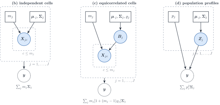
Panel (a), a mixture with a random cell label, is omitted. One specimen weights a covariance by a count or a fraction. A population profile puts a square on the fraction.
ii · A square weight shrinks the rare type’s contribution
viewof densCtrl = Inputs.form({
  v1: Inputs.range([1, 64], {value: 16, step: 1, label: "Variance, gene 1"}),
  v2: Inputs.range([1, 64], {value: 16, step: 1, label: "Variance, gene 2"}),
  rho1: Inputs.range([-0.85, 0.85], {value: 0.6, step: 0.05, label: "Correlation, type 1"}),
  rho2: Inputs.range([-0.85, 0.85], {value: 0, step: 0.05, label: "Correlation, type 2"}),
  proportion: Inputs.range([0.02, 0.98], {value: 0.5, step: 0.01, label: "Proportion of type 1"}),
  distance: Inputs.range([0, 16], {value: 2 * Math.SQRT2, step: 0.1, label: "Distance between centroids"})
})
// Axes stay at the slider extremes. A larger variance or a wider
// separation changes the shape, not the frame.
densModel = {
const p = densCtrl.proportion;
const S1 = mixLin.mat(densCtrl.v1, densCtrl.v2, densCtrl.rho1);
const S2 = mixLin.mat(densCtrl.v1, densCtrl.v2, densCtrl.rho2);
const u = 1 / Math.SQRT2;
const shift = densCtrl.distance / 2 * u;
const mu1 = [21 - shift, 21 + shift];
const mu2 = [21 + shift, 21 - shift];
const mean = [p * mu1[0] + (1 - p) * mu2[0], p * mu1[1] + (1 - p) * mu2[1]];
const { Squad, Slin } = mixLin.laws(p, S1, S2);
const vMax = 64, rhoMax = 0.85, dMax = 16;
const reach = 2 * Math.sqrt(vMax * (1 + rhoMax));
const half = dMax / (2 * Math.SQRT2);
const pad = 2;
const peak = (S) => 1 / (2 * Math.PI * Math.sqrt(Math.max(mixLin.det(S), 1e-12)));
const H = p <= 0 || p >= 1 ? 0 : -p * Math.log2(p) - (1 - p) * Math.log2(1 - p);
return {
Squad, Slin, S1, S2, mu1, mu2, mean, p, H,
colourMax: Math.max(peak(Squad), peak(Slin)),
xdom: [21 - half - reach - pad, 21 + half + reach + pad],
ydom: [21 - half - reach - pad, 21 + half + reach + pad]
};
}// Filled pixels: the density of the bulk law. Outlines: each type's own
// covariance, one standard deviation, centred on that type's mean.
densPanel = (model, law) => {
const quad = law === "quad";
const sum = quad ? model.Squad : model.Slin;
const colour = quad ? "#c45c26" : "#1d4e89";
const types = [
{ S: model.S1, colour: "#5c3d7a", mu: model.mu1, label: "Type 1" },
{ S: model.S2, colour: "#0e4d3a", mu: model.mu2, label: "Type 2" }
];
const viridis = (t) => {
const stops = [[68, 1, 84], [59, 82, 139], [33, 145, 140], [94, 201, 98], [253, 231, 37]];
const x = Math.max(0, Math.min(1, t)) * (stops.length - 1);
const i = Math.min(stops.length - 2, Math.floor(x));
const f = x - i;
const c = stops[i].map((v, k) => Math.round(v + f * (stops[i + 1][k] - v)));
return `rgb(${c[0]},${c[1]},${c[2]})`;
};
const W = 460, Ht = 210, left = 36, right = 8, top = 18, bottom = 22;
const x = d3.scaleLinear().domain(model.xdom).range([left, W - right]);
const y = d3.scaleLinear().domain(model.ydom).range([Ht - bottom, top]);
const svg = d3.create("svg").attr("viewBox", [0, 0, W, Ht]).attr("width", "100%")
.style("font", "13px sans-serif");
const nx = 56, ny = 36;
const Si = mixLin.inv(sum);
const detS = Math.max(mixLin.det(sum), 1e-12);
const norm = 1 / (2 * Math.PI * Math.sqrt(detS));
const dx = (model.xdom[1] - model.xdom[0]) / nx;
const dy = (model.ydom[1] - model.ydom[0]) / ny;
for (let i = 0; i < nx; i++) {
for (let j = 0; j < ny; j++) {
const x0 = model.xdom[0] + i * dx;
const y0 = model.ydom[0] + j * dy;
const r = [x0 + dx / 2 - model.mean[0], y0 + dy / 2 - model.mean[1]];
const f = norm * Math.exp(-0.5 * mixLin.quad(r, Si));
svg.append("rect")
.attr("x", x(x0)).attr("y", y(y0 + dy))
.attr("width", Math.max(0, x(x0 + dx) - x(x0)) + 0.4)
.attr("height", Math.max(0, y(y0) - y(y0 + dy)) + 0.4)
.attr("fill", viridis(f / model.colourMax))
.attr("stroke", "none");
}
}
svg.append("g").attr("transform", `translate(${left},0)`).call(d3.axisLeft(y).ticks(4));
svg.append("g").attr("transform", `translate(0,${Ht - bottom})`).call(d3.axisBottom(x).ticks(4));
const line = d3.line().x((d) => x(d[0])).y((d) => y(d[1]));
for (const t of types) {
svg.append("path")
.attr("d", line(mixLin.ring(t.mu, t.S, 1, 64)) + "Z")
.attr("fill", "none").attr("stroke", t.colour).attr("stroke-width", 2);
svg.append("circle").attr("cx", x(t.mu[0])).attr("cy", y(t.mu[1])).attr("r", 4).attr("fill", t.colour);
}
svg.append("circle").attr("cx", x(model.mean[0])).attr("cy", y(model.mean[1]))
.attr("r", 3.5).attr("fill", colour).attr("stroke", "#f7f4ef");
svg.append("text").attr("x", left + 6).attr("y", 16).attr("fill", colour).attr("font-weight", 700)
.text(quad ? "Population density, weights p² and (1 − p)²" : "Single-cell density, weights p and 1 − p");
return svg.node();
}The proportion of type 1 is the weight in each panel. Filled pixels are the bulk density, population weights on the left and single-cell weights on the right, on one colour scale. Outlines are each type’s own covariance, one standard deviation, on that type’s mean. The axes stay fixed.
iii · The square weight is not the wider interval
viewof ciCtrl = Inputs.form({
  v1: Inputs.range([1, 64], {value: 16, step: 1, label: "Variance, gene 1"}),
  v2: Inputs.range([1, 64], {value: 16, step: 1, label: "Variance, gene 2"}),
  rho: Inputs.range([-0.85, 0.85], {value: 0.6, step: 0.05, label: "Correlation, type 1"}),
  proportion: Inputs.range([0.02, 0.98], {value: 0.05, step: 0.01, label: "True proportion of type 1"})
})ciChart = {
const p0 = ciCtrl.proportion;
const mu1 = [20, 22], mu2 = [22, 20];
const delta = [mu1[0] - mu2[0], mu1[1] - mu2[1]];
const meanOf = (p) => [p * mu1[0] + (1 - p) * mu2[0], p * mu1[1] + (1 - p) * mu2[1]];
const S1 = mixLin.mat(ciCtrl.v1, ciCtrl.v2, ciCtrl.rho);
const S2 = mixLin.mat(ciCtrl.v1, ciCtrl.v2, 0);
const at = (p) => mixLin.laws(p, S1, S2);
const base = at(p0);
const mean0 = meanOf(p0);
let y = mean0;
if (ciDraw) {
const z1 = mixLin.normal(20261112 + 2 * ciDraw);
const z2 = mixLin.normal(20261112 + 2 * ciDraw + 1);
const L00 = Math.sqrt(Math.max(base.Slin[0][0], 1e-12));
const L10 = base.Slin[1][0] / L00;
const L11 = Math.sqrt(Math.max(base.Slin[1][1] - L10 * L10, 1e-12));
y = [mean0[0] + L00 * z1, mean0[1] + L10 * z1 + L11 * z2];
}
const fq = mixLin.fisher(delta, base.Squad, base.SpQuad);
const fl = mixLin.fisher(delta, base.Slin, base.SpLin);
const grid = d3.range(0.02, 0.981, 0.01);
const series = [
{ name: "Population", colour: "#c45c26", half: fq.half, cov: (p) => at(p).Squad },
{ name: "Single cell", colour: "#1d4e89", half: fl.half, cov: (p) => at(p).Slin }
];
for (const s of series) {
s.ll = grid.map((p) => mixLin.loglik(y, meanOf(p), s.cov(p)));
s.max = Math.max(...s.ll);
}
const W = 980, H = 250, mid = 500;
const svg = d3.create("svg").attr("viewBox", [0, 0, W, H]).attr("width", "100%")
.style("font", "14px sans-serif");
const xShare = d3.scaleLinear().domain([0, 1]).range([48, mid - 24]);
svg.append("text").attr("x", 48).attr("y", 16).attr("fill", "#1c2b24").attr("font-weight", 700)
.text("Wald interval for the true proportion");
svg.append("line").attr("x1", xShare(0)).attr("x2", xShare(1)).attr("y1", 108).attr("y2", 108)
.attr("stroke", "#cfc6b8");
svg.append("line").attr("x1", xShare(p0)).attr("x2", xShare(p0)).attr("y1", 36).attr("y2", 168)
.attr("stroke", "#1c2b24").attr("stroke-dasharray", "4 3");
series.forEach((s, i) => {
const y0 = 78 + i * 48;
const lo = Math.max(0, p0 - s.half), hi = Math.min(1, p0 + s.half);
svg.append("line").attr("x1", xShare(lo)).attr("x2", xShare(hi)).attr("y1", y0).attr("y2", y0)
.attr("stroke", s.colour).attr("stroke-width", 8).attr("stroke-linecap", "round");
svg.append("circle").attr("cx", xShare(p0)).attr("cy", y0).attr("r", 4).attr("fill", "#1c2b24");
svg.append("text").attr("x", 48).attr("y", y0 - 12).attr("fill", s.colour)
.text(`${s.name}: half-width ${s.half.toFixed(2)}`);
});
svg.append("text").attr("x", 48).attr("y", 200).attr("fill", "#5c6b63")
.text("Dashed line: true proportion. Bars are clipped to [0, 1].");
const xP = d3.scaleLinear().domain([0.02, 0.98]).range([mid + 36, W - 16]);
const lls = series.flatMap((s) => s.ll);
const cuts = series.map((s) => s.max - 1.92);
const yL = d3.scaleLinear()
.domain([Math.min(...lls, ...cuts), Math.max(...lls)])
.range([H - 36, 28])
.nice();
svg.append("text").attr("x", mid + 36).attr("y", 16).attr("fill", "#1c2b24").attr("font-weight", 700)
.text(ciDraw ? "Log-likelihood of the drawn bulk" : "Log-likelihood at the mean bulk");
svg.append("g").attr("transform", `translate(${mid + 36},0)`).call(d3.axisLeft(yL).ticks(4));
svg.append("g").attr("transform", `translate(0,${H - 36})`).call(d3.axisBottom(xP).ticks(5));
const panel = svg.append("g").attr("clip-path", "url(#ll-clip)");
svg.append("clipPath").attr("id", "ll-clip").append("rect")
.attr("x", mid + 8).attr("y", 20).attr("width", W - mid - 8).attr("height", H - 56);
const line = d3.line().x((d, i) => xP(grid[i])).y((d) => yL(d));
for (const s of series) {
panel.append("path").attr("d", line(s.ll)).attr("fill", "none")
.attr("stroke", s.colour).attr("stroke-width", 2);
const cut = s.max - 1.92;
panel.append("line").attr("x1", xP(0.02)).attr("x2", xP(0.98))
.attr("y1", yL(cut)).attr("y2", yL(cut))
.attr("stroke", s.colour).attr("stroke-dasharray", "3 3").attr("opacity", 0.85);
}
return svg.node();
}Expected Fisher information of one Gaussian bulk: the mean contrast \(\delta=\mu_1-\mu_2\), plus half the trace of \(\Sigma^{-1}\Sigma'\Sigma^{-1}\Sigma'\). Opening setting, checked separately: variances 16, correlation 0.6 against 0, proportion 0.05, half-widths 0.92 (square) and 2.09 (linear). The square weight is tighter because \(p^2+(1-p)^2\) still moves. The dashed lines on the right are the likelihood-ratio cuts, 1.92 below each maximum, which is 3.84 on the deviance scale.
2 · From one cell to the bulk
i · Symbols for the averaged mixture
| Symbol | Meaning on the next two slides |
|---|---|
| \(p_{ji}\) | Cell fraction of type \(j\) in bulk \(i\) |
| \(n_i\) | Number of cells behind that bulk |
| \(a_i\) | capture ratio from the reference to the bulk |
| \(c_i = a_i n_i\) | Scale of the mean |
| \(\phi_i = a_i^2 n_i\) | Scale of the within-type covariance |
| \(\boldsymbol{S}_W(\boldsymbol{p}) = \sum_j p_j \boldsymbol{\Sigma}_{W,j}\) | Linear mixture of within-type covariances |
| \(\boldsymbol{D}_i\) | Diagonal noise added by the bulk |
Per-cell means wear a tilde. \(\boldsymbol{\Sigma}_{W,j}\) is the cell-to-cell covariance of one specimen.
ii · Three layers, from a missing count to a diagonal
The per-cell average
\[\tilde{\boldsymbol{y}}\mid\boldsymbol{p},n\sim\mathcal{N}\!\left(\tilde{\boldsymbol{\mu}}\boldsymbol{p},\,n^{-1}\boldsymbol{S}_W(\boldsymbol{p})\right)\]
\(n\) is missing. It can come from the covariance magnitude, from a paired bulk, or from an external count.
Two scales
\[\boldsymbol{y}\mid\boldsymbol{p},a,n\sim\mathcal{N}\!\left(c\,\tilde{\boldsymbol{\mu}}\boldsymbol{p},\,\phi\,\boldsymbol{S}_W(\boldsymbol{p})\right)\]
\[c = an,\qquad \phi = a^{2}n\]
The simplex lets the mean pin \(c\). \(\phi\) is what is left in the covariance.
A diagonal the bulk adds
\[\boldsymbol{\Sigma}=\phi\,\boldsymbol{S}_W(\boldsymbol{p})+\boldsymbol{D}\]
The off-diagonal entries pin \(\phi\). The diagonal excess is \(\boldsymbol{D}\).
The raw \(\boldsymbol{\Sigma}_{W,j}\) matches the bulk only at capture ratio 1. Otherwise the bulk adds its own diagonal. This fit does not use that diagonal.
iii · Measurement, then expression
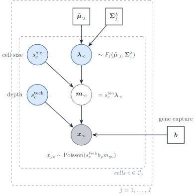
\(\boldsymbol{\lambda}_{\cdot c}\) is the size-free expression. \(s^{\mathrm{bio}}\), \(s^{\mathrm{tech}}\) and \(\boldsymbol{b}\) are measurement. Sarkar and Stephens, and Fang and Pachter, separate the two. The \(\lambda\) of the covariance slides is the shrinkage intensity, a different quantity.
iv · UMIs make the measurement Poisson
\[x_{gc}\sim\mathrm{Poisson}\bigl(s^{\mathrm{tech}}_c\, b_g\, m_{gc}\bigr)\]
- Inside one protocol, \(b_g\) is absorbed into the reference. It cancels from a within-protocol contrast.
- Between the reference and the bulk it need not cancel. That ratio is the gene scale the benchmark tried, and did not keep.
- Spike-in controls in those papers put the extra variance in the expression, not in the capture.
v · What the sample covariance mixes
The sample covariance of raw UMI counts mixes three objects. Only part of it belongs in the bulk.
- The Poisson diagonal is single-cell sampling, at single-cell depth. A bulk has its own sampling noise.
- The technical size factor is a protocol artefact. It correlates every gene with every other gene.
- The biological size factor belongs in the bulk. Cells differ in volume, and the tissue sums them as they are.
vi · What the winning row keeps
- Gaussian likelihood on the raw counts, with the linear weight. The Poisson diagonal stays in the plug-in.
- Denoising that diagonal is the weak row: RMSE 0.47 at 96 h on the Welch panel, a wrong split inside the mesoderm lineage.
- A Poisson–log-normal convolution, integrating the expression noise instead of plugging in two moments, is an extension. It is not a row of this benchmark.
vii · Capture and depth are different powers of \(a\)
scaleCloud = {
  const a = 10 ** scaleCtrl.a;
  const n = 10 ** scaleCtrl.n;
  const p = 0.35;
  const phi = a * a * n;
  const S1 = mixLin.mat(16, 16, 0.5);
  const S2 = mixLin.mat(16, 16, 0);
  const Sw = mixLin.add(S1, S2, p, 1 - p);
  const Sbio = mixLin.add(Sw, [[0, 0], [0, 0]], phi, 0);
  const aMax = 10 ** 0.7, nMax = 10 ** 4;
  const reach = 2 * Math.sqrt(aMax * aMax * nMax * 16);
  const W = 520, H = 280, m = 42;
  const x = d3.scaleLinear().domain([-reach, reach]).range([m, W - 8]);
  const y = d3.scaleLinear().domain([-reach, reach]).range([H - 28, 22]);
  const svg = d3.create("svg").attr("viewBox", [0, 0, W, H]).attr("width", "100%").style("font", "14px sans-serif");
  const line = d3.line().x((d) => x(d[0])).y((d) => y(d[1]));
  svg.append("path").attr("d", line(mixLin.ring([0, 0], Sbio, 2, 80)) + "Z")
    .attr("fill", "#1d4e89").attr("fill-opacity", 0.28).attr("stroke", "#1d4e89");
  svg.append("text").attr("x", m).attr("y", 16).attr("fill", "#1c2b24")
    .text("φ S_W only. The axes stay at the slider extremes.");
  return svg.node();
}
scaleRead = {
const a = 10 ** scaleCtrl.a;
const n = 10 ** scaleCtrl.n;
const c = a * n, phi = a * a * n;
const box = (label, value) => `<div style="margin:0.35em 0"><span style="color:#5c6b63">${label}</span><br><b style="font-size:22px;color:#0e4d3a">${value}</b></div>`;
return html`<div style="font-size:15px;line-height:1.25">${box("Mean scale c = a n", c.toPrecision(3))}${box("Variance scale φ = a² n", phi.toPrecision(3))}</div>`;
}Proportion of type 1 fixed at 0.35. Variances 16. Type 1 correlation 0.5, type 2 correlation 0. The ellipse is \(\phi\boldsymbol{S}_W\) only. The fitted model does not add a diagonal.
viii · The best fit profiles out two scales and nothing else
| Technical factor | In the raw-covariance fit at \(\lambda = 0.5\) |
|---|---|
| Mean scale \(c\) | Used. Profiled out in closed form |
| Variance scale \(\phi\) | Used. Profiled out in closed form; fitted values \(10^{6}\) to \(10^{8}\) |
| Cell count \(n\) and capture \(a\), separately | Not fitted. \(\hat n = c^{2}/\phi\) is below one cell |
| Diagonal \(\boldsymbol{D}\) | Not used. A gene-wise variance scale did not converge in 13 of 18 chains |
| Gene scale \(b_g\) on the bulk | Not used. It helps on the small panels and hurts on the Welch panel at 96 h |
| Library-size normalisation | None. Raw counts on both sides |
The covariance plug-in is the raw covariance of each type, with its off-diagonal terms multiplied to reach \(\lambda = 0.5\); variances are untouched. Of the three layers, the fit keeps the second.
3 · Which genes
i · The authors’ cell filters stand
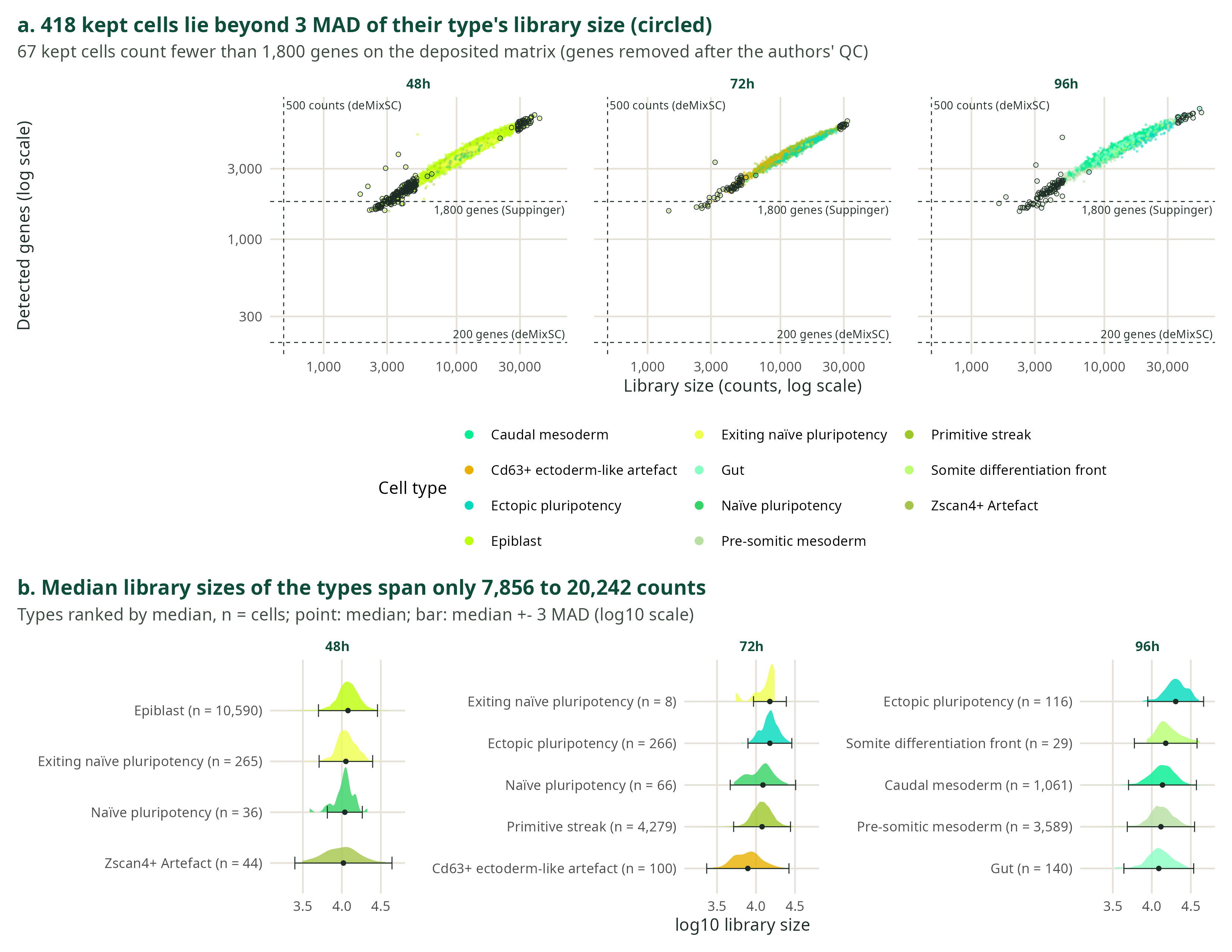
Cells kept above 1,800 genes and below 10% mitochondrial counts stay kept. Genes whose non-zero entries are more than 90% fractional are dropped. That fractional cut is not a detection rule. The presence gate is the detection rule, and it is the next slide.
ii · Two detection rules, and neither contains the other
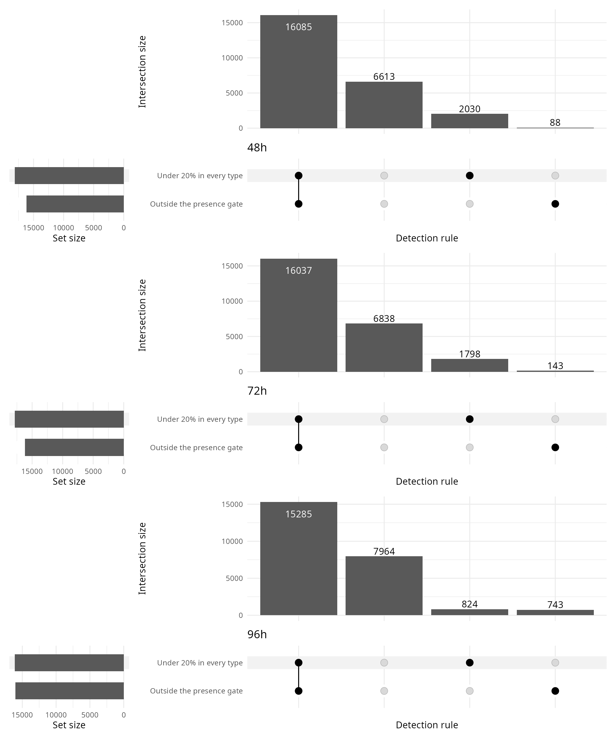
Outside the presence gate: under 5% of the cells of some scored type, or zero within-type variance. Under 20% in every type: no scored type reaches that rate. deMixSC at 5% of all cells is not drawn, because those genes are already outside the presence gate. All-zero genes, and the mitochondrial, ribosomal and Gm rules, are already absent.
iii · At 48 h the same scores, by type and by cell line
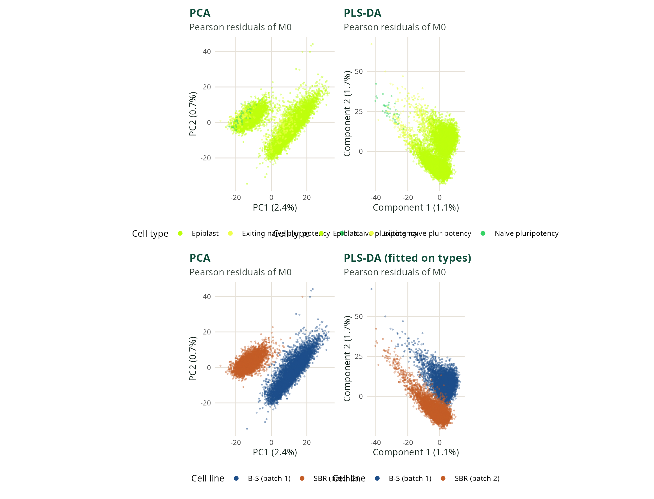
Pearson residuals of \(M_0\), two components, cell type as the response. The lower row colours the same scores by cell line.
iv · At 72 h the projection is by cell type
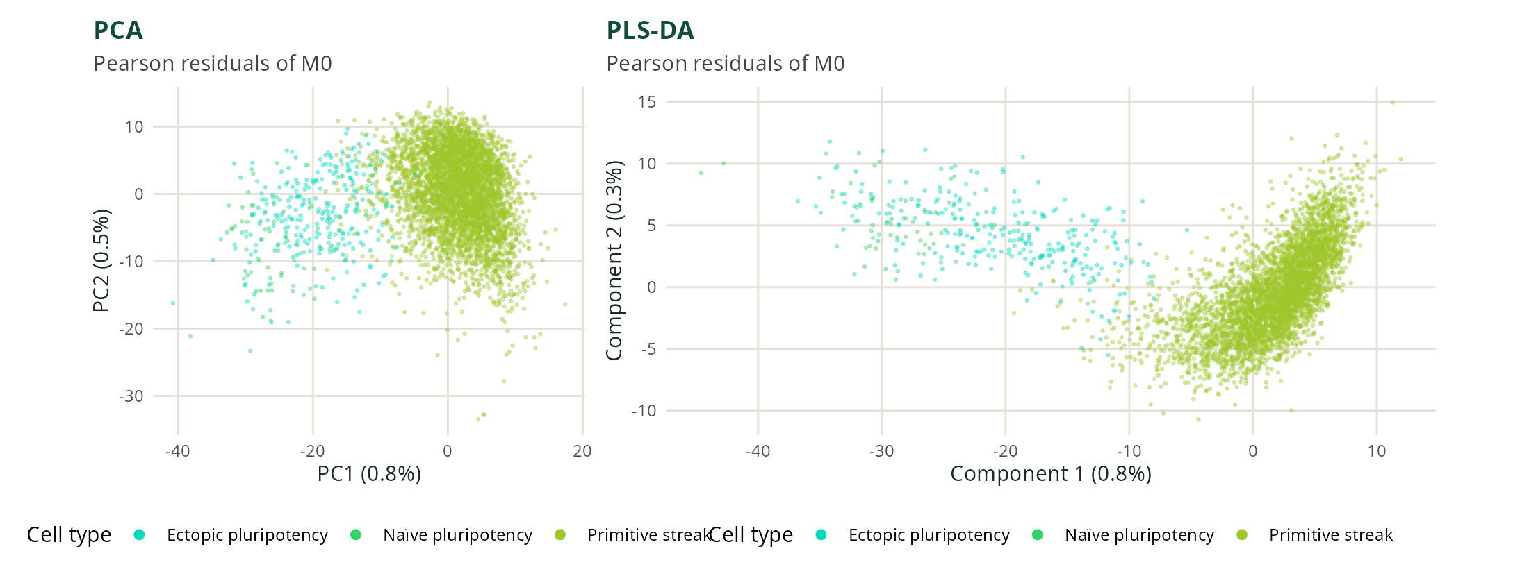
One cell line at 72 h. Same residuals, same two components, cell type as the response.
v · At 96 h the projection is by cell type
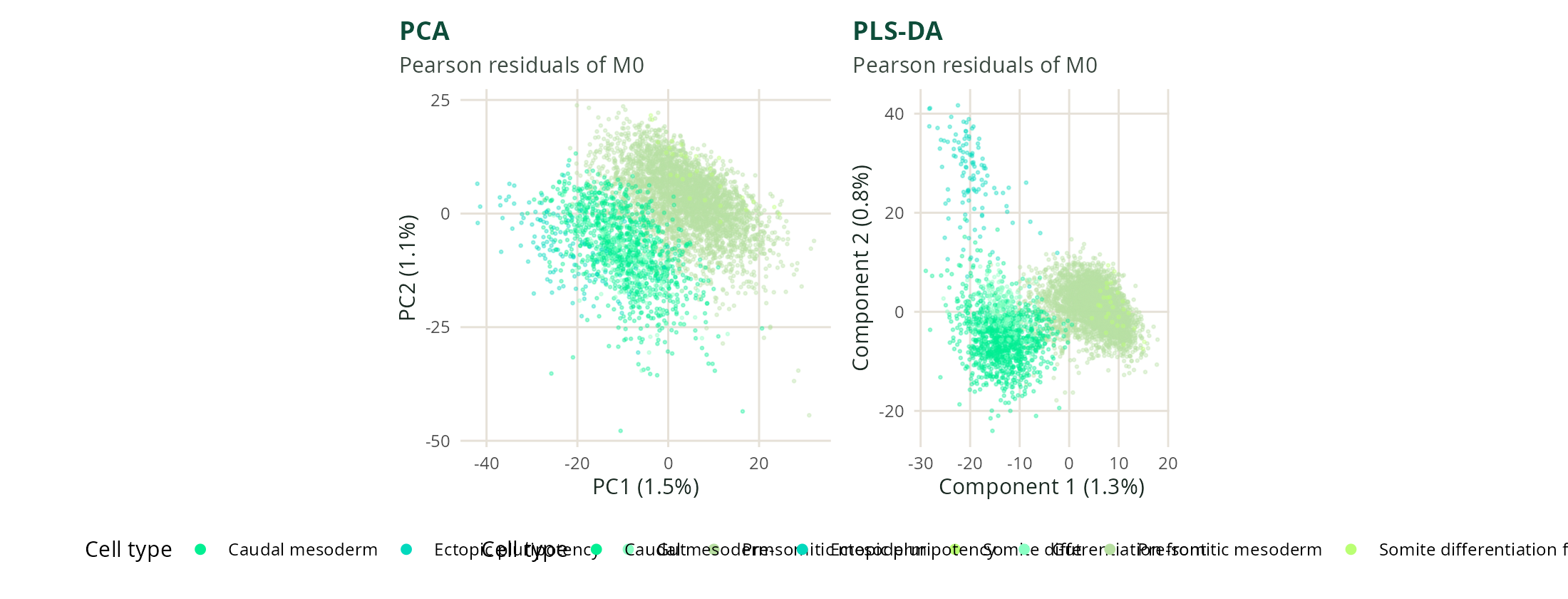
One cell line at 96 h. Same construction as the 72 h slide.
vi · Three of the four tests assume independent cells
| Test | Reference law | What has to be true |
|---|---|---|
| Likelihood ratio | \(\chi^2_{J-1}\) on the deviance | Negative-binomial mean and dispersion, dispersion treated as known, independent cells |
| ANOVA on the shifted log | \(F_{J-1,\,C-J}\) | Independent normal cells after \(\log(x/s+y_0)\) |
| Quasi-likelihood \(F\) | \(F\), dispersion estimated | Extra-Poisson variance is allowed; cells are still independent |
| Permuted Welch \(G\) | Freedman–Lane label permutation | Residuals of the null model are exchangeable within batch; type variances may differ |
The first three refer a sum of squares, or a deviance, to a table that independence justifies. Only the permutation uses the residual cloud.
vii · At 48 h the analytic tests read cell line as type
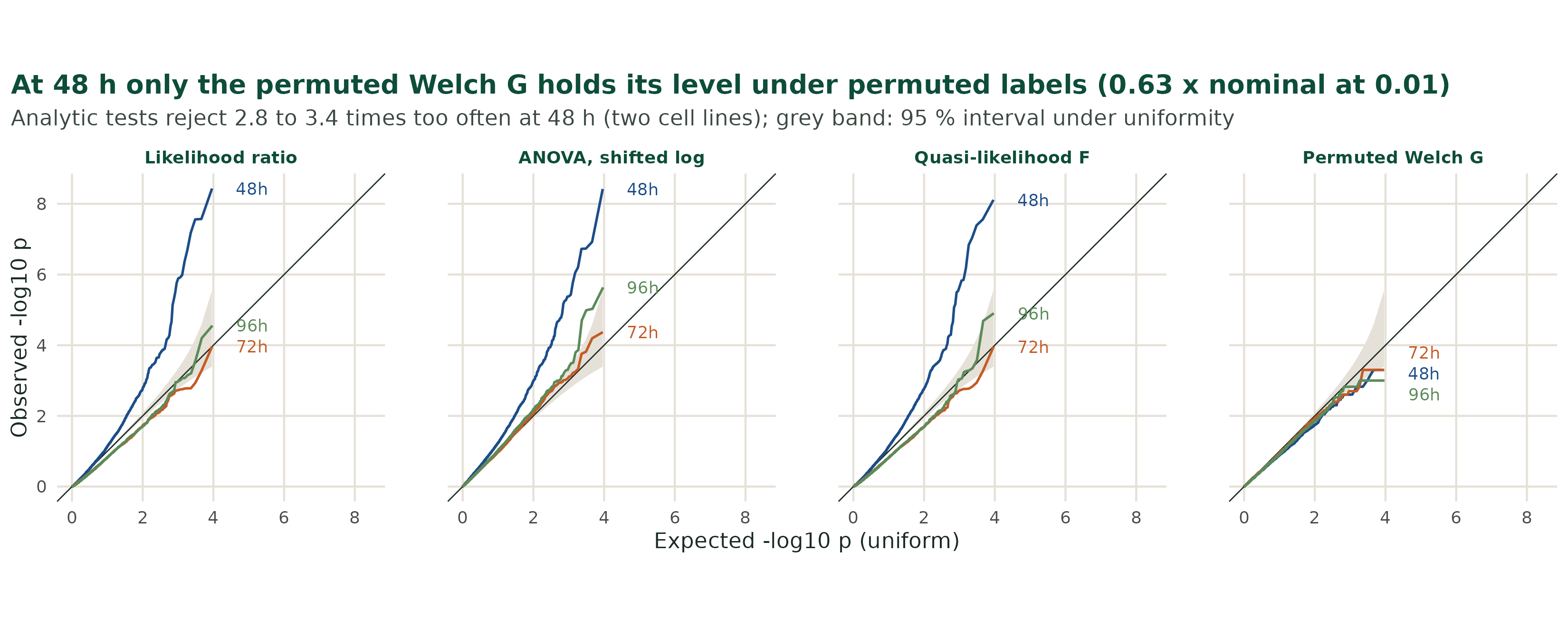
At the 0.01 level and at 48 h, the likelihood ratio rejects 2.9 times the nominal rate, the quasi-likelihood \(F\) 2.8 times, and the shifted-log ANOVA 3.4 times. The permuted Welch \(G\) rejects 0.63 times. A within-batch permutation keeps the cell-line shift, and the analytic tests do not model the cell line.
viii · Dispersion widens two intervals; correlation fools the within-cell ones
forestChart = {
  const phi = forestCtrl.phi, rho = forestCtrl.rho;
  const n1 = 40, n2 = 10, ratio = 4, s0 = 20, delta = 1, mu1 = 20, mu2 = 21;
  const m1 = phi * s0, m2 = ratio * m1;
  const v1 = m1 * (1 - rho), v2 = m2 * (1 - rho);
  const trueSe = Math.sqrt(
    m1 * (1 + (n1 - 1) * rho) / n1 + m2 * (1 + (n2 - 1) * rho) / n2
  );
  const poisSe = Math.sqrt(mu1 / n1 + mu2 / n2);
  const sp2 = ((n1 - 1) * v1 + (n2 - 1) * v2) / (n1 + n2 - 2);
  const rows = [
    { name: "Likelihood ratio", se: Math.sqrt(s0 / n1 + s0 / n2), colour: "#5c3d7a" },
    { name: "ANOVA, pooled", se: Math.sqrt(sp2 * (1 / n1 + 1 / n2)), colour: "#c45c26" },
    { name: "Quasi-likelihood", se: Math.sqrt(phi) * poisSe, colour: "#1d4e89" },
    { name: "Welch, within type", se: Math.sqrt(v1 / n1 + v2 / n2), colour: "#0e4d3a" }
  ];
  const Phi = (z) => {
    const t = 1 / (1 + 0.2316419 * Math.abs(z));
    const d = 0.3989422804 * Math.exp(-0.5 * z * z);
    const p = d * t * (0.319381530 + t * (-0.356563782 + t * (1.781477937 + t * (-1.821255978 + t * 1.330274429))));
    return z >= 0 ? 1 - p : p;
  };
  const coverP = (se) => 2 * Phi(1.96 * se / trueSe) - 1;
  const draws = Math.max(forestDraw, 0);
  const hits = rows.map(() => 0);
  let dHat = delta;
  for (let b = 1; b <= Math.max(draws, 1); b++) {
    const z = mixLin.normal(20261112 + b);
    const centre = delta + trueSe * z;
    if (b === Math.max(draws, 1)) dHat = centre;
    if (draws > 0) {
      rows.forEach((r, i) => {
        if (Math.abs(centre - delta) <= 1.96 * r.se) hits[i] += 1;
      });
    }
  }
  const halfRange = Math.max(8, 1.96 * trueSe * 1.25);
  const W = 980, H = 250, left = 168, right = 150;
  const x = d3.scaleLinear().domain([delta - halfRange, delta + halfRange]).range([left, W - right]);
  const svg = d3.create("svg").attr("viewBox", [0, 0, W, H]).attr("width", "100%").style("font", "14px sans-serif");
  svg.append("line").attr("x1", x(delta)).attr("x2", x(delta)).attr("y1", 16).attr("y2", H - 28)
    .attr("stroke", "#1c2b24").attr("stroke-dasharray", "4 3");
  svg.append("line")
    .attr("x1", x(delta - 1.96 * trueSe)).attr("x2", x(Math.min(delta + halfRange, delta + 1.96 * trueSe)))
    .attr("y1", 28).attr("y2", 28).attr("stroke", "#cfc6b8").attr("stroke-width", 10);
  rows.forEach((r, i) => {
    const y = 62 + i * 42;
    const lo = dHat - 1.96 * r.se, hi = dHat + 1.96 * r.se;
    svg.append("line").attr("x1", x(lo)).attr("x2", x(hi)).attr("y1", y).attr("y2", y)
      .attr("stroke", r.colour).attr("stroke-width", 6).attr("stroke-linecap", "round");
    svg.append("circle").attr("cx", x(dHat)).attr("cy", y).attr("r", 4).attr("fill", r.colour);
    svg.append("text").attr("x", 8).attr("y", y + 4).attr("fill", r.colour).text(r.name);
    const tally = draws > 0 ? `, ${hits[i]}/${draws} draws` : "";
    svg.append("text").attr("x", W - 8).attr("y", y + 4).attr("text-anchor", "end").attr("fill", "#5c6b63")
      .text(`${(100 * coverP(r.se)).toFixed(0)}%${tally}`);
  });
  svg.append("text").attr("x", left).attr("y", H - 8).attr("fill", "#5c6b63")
    .text("Grey: true 95% interval. Dashed: true difference, 1.");
  return svg.node();
}
A Gaussian sketch, not the Suppinger likelihoods. Forty cells and ten cells. Type 2’s cell variance is four times type 1’s, and \(\varphi\) multiplies both. In the count model that factor is the negative binomial dispersion: variance \(\mu+\varphi\mu^{2}\), biological variability of the expression or of the size factor. For a Poisson point process over a long window, variance over mean tends to the Fano factor, and the extra above 1 is this dispersion. The capture is taken to be long enough for that regime. The likelihood-ratio interval uses a fixed variance. The quasi-likelihood interval multiplies the Poisson standard error by \(\sqrt{\varphi}\). ANOVA and Welch use within-type variances, which shrink as the correlation grows, while the variance of the mean grows. Definitions: Fano factor, Poisson point process.
4 · The covariance
i · A covariance entry is a property of the gene pair
- Deleting a gene leaves the other covariance entries as they were. A precision entry is a Schur complement of the panel, so it changes when a neighbour is removed.
- The likelihood inverts a sum of type covariances. That sum is dense even when every type precision is sparse.
- The shrinkage intensity spends variance against bias. The sparse precision estimators stay in the benchmark as sensitivity analyses, not as the plug-in.
ii · The closed form minimises the wrong risk
\[\hat\Sigma_{gg}=V_{gg},\qquad \hat\Sigma_{gg'}=(1-\lambda)\,R_{gg'}\sqrt{V_{gg}V_{g'g'}}\]
\[R(\lambda)=\mathbb{E}\bigl\|\hat{\boldsymbol{\Sigma}}(\lambda)-\boldsymbol{\Sigma}\bigr\|_{F}^{2}=\sum_{g,g'}\mathbb{E}\bigl(\hat\Sigma_{gg'}-\Sigma_{gg'}\bigr)^{2}\]
\(\lambda=0\) keeps the sample correlations. \(\lambda=1\) keeps only the variances, a bias toward no correlation. The closed form minimises the Frobenius risk. That minimum is a bias–variance trade-off on the covariance entries. This risk is not the deconvolution loss. DeCovarT’s selection criterion is a Gaussian log-density of held-out cells. That cell-wise score is written and has not been run. The reported level was read on the composition error.
- Welch panel, 96 h, mean over three standard-Wnt replicates: raw covariance at \(\lambda = 0.5\) has RMSE 0.034. The closed-form \(\lambda\) has RMSE 0.36.
- \(\lambda = 0.5\) is the best of the four levels \(0.25, 0.5, 0.75, 1\) on those same nine samples. It is the bulk-RMSE level, not a completed nested cross-validation. The 0.034 is optimistic.
iii · On the smallest panel, the three mesoderm profiles correlate at 0.97 and above
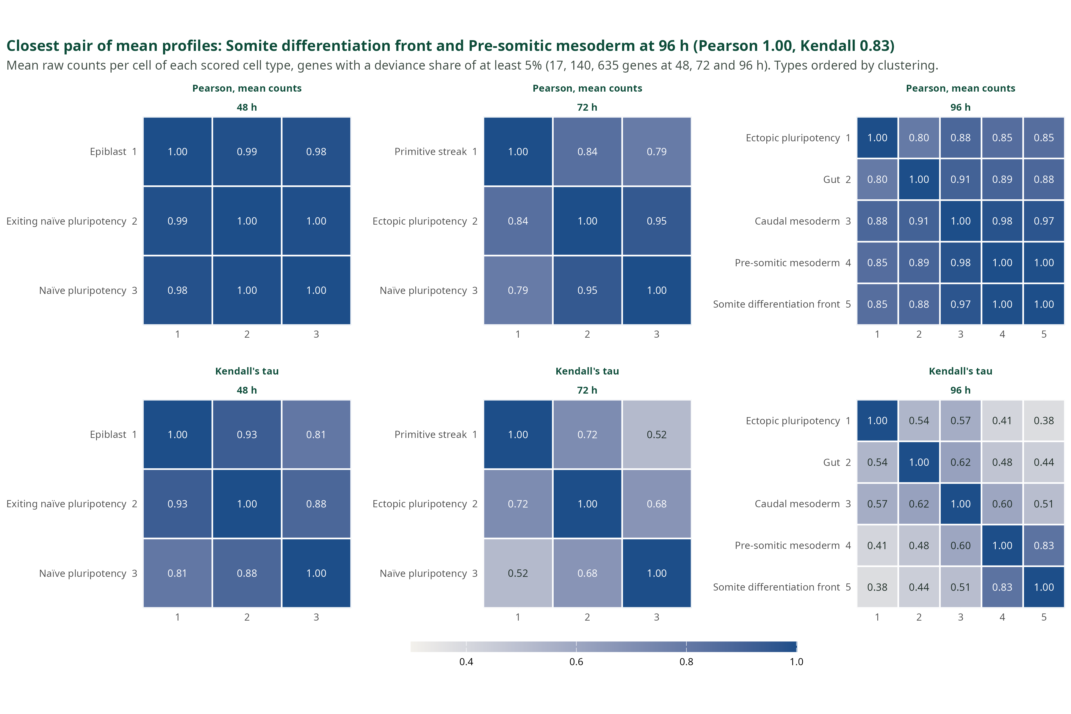
Genes whose type effect explains at least 5% of the deviance: 17, 140 and 635 genes at 48, 72 and 96 h. Top row: Pearson correlation of the mean raw counts per cell, the scale the solvers see. Bottom row: Kendall’s tau. Types are ordered by clustering. At 96 h: caudal against pre-somitic mesoderm 0.98, caudal against somite front 0.97, pre-somitic against somite front 1.00.
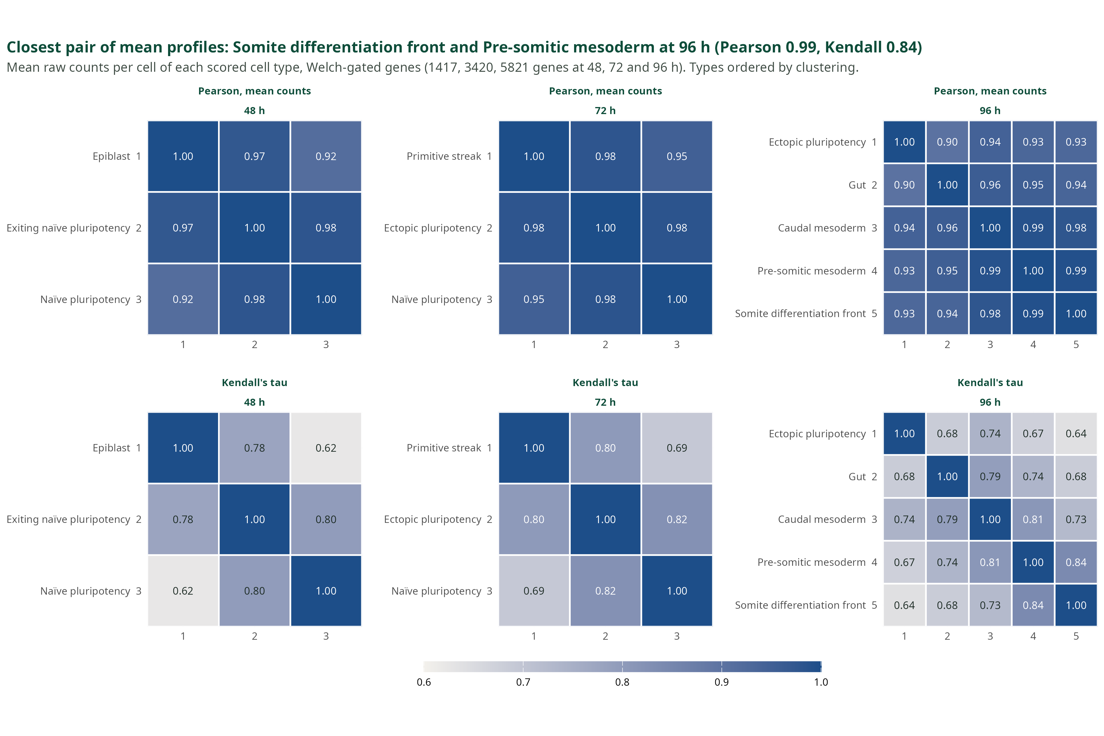
iv · On the Welch panel the mesoderm lineage stays at 0.98 to 0.99
- Unweighted least squares fails. On one 96 h sample, non-negative least squares gives 100% to caudal mesoderm, observed at 0.22, and nothing to pre-somitic mesoderm, observed at 0.73. With the full raw covariance as weight, the same programme returns 0.22 and 0.78.
- A condition number is the wrong gene filter here. It reads the mean signature only. Minimising it keeps the genes that separate distant lineages and drops those that split neighbours. This is an argument, not a measurement: no condition number was computed.
Welch-gated genes: 1,417, 3,420 and 5,821 at 48, 72 and 96 h. The cosine similarity of the closest pair is 0.98 at 48 h and 72 h and 0.99 at 96 h.
5 · The benchmark
i · Eight comparators, four ways to model the bulk
Click a paradigm to fold its methods. DeCovarT is a multivariate likelihood: the covariance of the bulk depends on the composition.
ii · Seven rungs, and where this benchmark sits
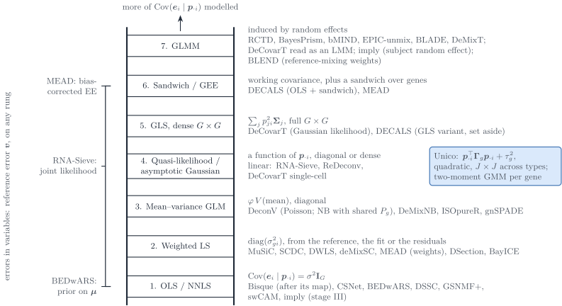
The vignette ladder, reduced to the slide. DeCovarT sits on the dense covariance. MEAD puts dependence in the sandwich. Weighted least squares are diagonal.
iii · Same likelihood, and the plug-in decides the error
| DeCovarT variant | Welch panel, 96 h, or what the figure states |
|---|---|
| Raw covariance, \(\lambda = 0.5\), L-BFGS-B | RMSE 0.034. Best of the four levels, on the samples that score it |
| Raw covariance, closed-form \(\lambda\) | RMSE 0.36 |
| Denoised covariance | RMSE 0.47 |
| Newton against L-BFGS-B | Largest RMSE gap on the figure: 0.321 |
| Bulk divided by the gene scale \(b_g\) | The figure’s own summary: mean RMSE 0.18, against 0.31 on the bulk as is |
Blue on the next two figures is trust-region Newton. Orange is L-BFGS-B. Black is a comparator, or the quadratic programme of the multivariate RNA-Sieve.
iv · Root mean squared error, three replicates
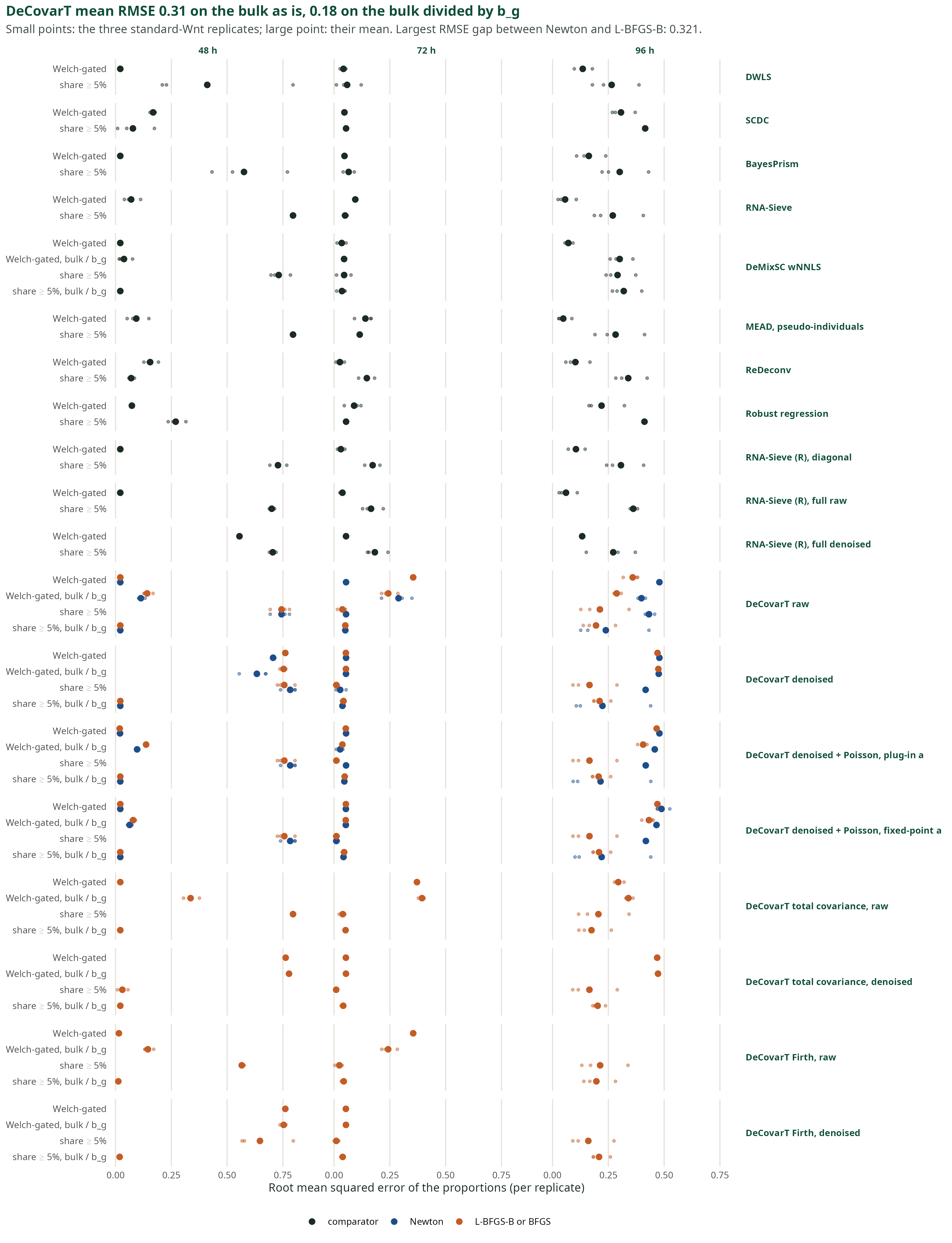
Small points: the three standard-Wnt replicates. Large point: their mean. Rows are methods. Columns are the bulk times.
v · Aitchison distance ranks the rare types
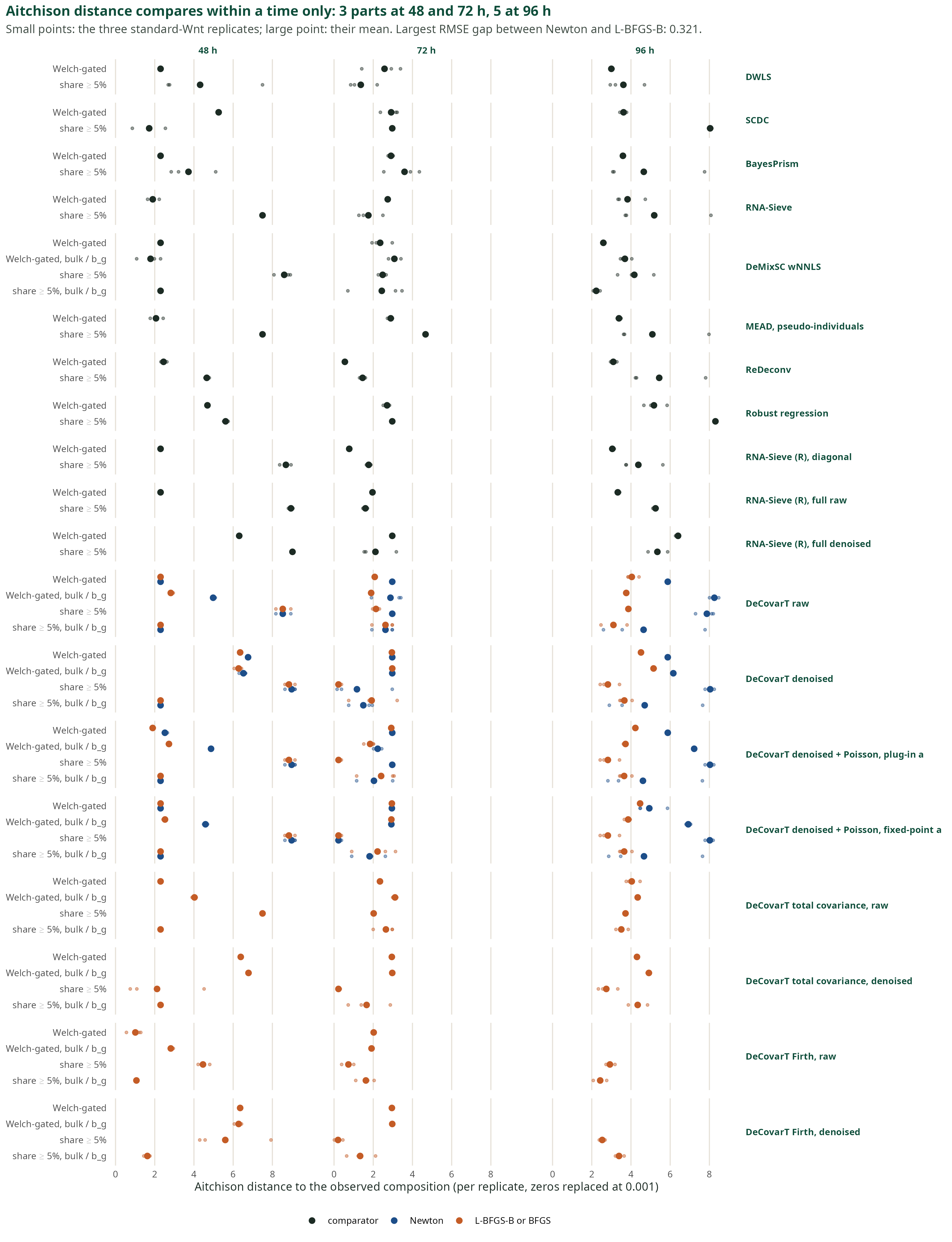
Compare methods inside one time only: 3 parts at 48 h and 72 h, 5 parts at 96 h. Zeros are replaced at 0.001 before the centred log-ratio. A rare type set to zero costs more here than a shift between two abundant types, so this is not a copy of the RMSE ranking.
vi · What this benchmark supports
- The penalty on the covariance moves the error more than the choice of optimiser: 0.36 against 0.034 at 96 h on the Welch panel.
- The fit is not missing the mode. Its likelihood beats the observed composition in all 36 cases.
- A quadratic programme on the same raw plug-ins reaches RMSE 0.060. The plug-in, not the solver, is the gap.
- Refining the mean profiles from one bulk raises the error to about 0.50.
- Summing caudal mesoderm, pre-somitic mesoderm and the somite front at 96 h puts twelve of thirteen methods at 0.04 or below.
\(\lambda = 0.5\) is the bulk-RMSE level on the samples that define the error. The cell-wise nested score has not chosen it. That score is still required before the row is compared with MEAD or RNA-Sieve.
6 · What remains
i · Five directions, ranked by this evidence
- Choose the shrinkage level without the answer. Score each level on pseudo-bulks of held-out cells. Compare one common level with one per type.
- Estimate the composition from the mean equation. Keep the covariance as a weight, and take the variance from a jackknife over gene clusters.
- Treat close types as a lineage. Fit the lineage first, then its split. This helps every method.
- Add a measurement layer between bulk and reference. A mean–variance law per gene across bulks.
- Carry the precision of the reference. Replicates or a delete-a-group jackknife, instead of refitting the reference from the bulk.
Which direction matters most depends on the regime. Three indicators were measured: cosine similarity of the profiles, bulk-to-reference shift, cells per gene. Covariance changes between conditions cannot be measured, because the reference follows one protocol.
ii · An aliquot is the external check
The Suppinger reference is not a split of the bulk. An aliquot is a physical split of one specimen, so the bulk and the single-cell library measure the same material.
- Dong and colleagues, 10.1093/bib/bbz166. Mouse mammary suspension, GEO GSE136148. SCDC, already a comparator, was published on that split. Two animals. The truth is the single-cell recovery.
- Guo and colleagues, 10.1101/gr.278822.123. Healthy retina, 24 specimens, same nuclei suspension. DeMixSC, already a comparator. Bulk GSE175937.
- Dai and colleagues, 10.1126/sciadv.adh2588, on Jourdon and colleagues, 10.1038/s41593-023-01399-0. About 60 forebrain-organoid samples at TD0, TD30 and TD60. A preparation may pool organoids. Access is NIMH Data Archive study 1482.
He and colleagues and the BEDwARS analysis of Ghaffari and colleagues are not split aliquots. A usable set needs traceable identifiers, a published deconvolution, and an independent count when the single-cell recovery would be the only truth.
iii · How is a rare type weighted?
- By the cell count under both laws
- By \(p^{2}\) under the population law and by \(p\) under the single-cell law
- By \(p\) under both laws
- Not at all, once the types are independent
iv · What chose \(\lambda = 0.5\)?
- The nested score on held-out cells
- The best composition error on the scored samples; the cell-wise nested score has not chosen it
- The closed form of the Frobenius risk
- A match of pseudo-bulks to the real bulks
v · Where does \(b_g\) cancel?
- Between the reference and the bulk, always
- Inside one protocol. It need not cancel between the reference and the bulk
- It never cancels, with or without UMIs
- Only after library-size normalisation
Appendix: three optimisers for the same likelihood
Trust-region Newton
\[\Delta=\arg\max_{\lVert\Delta\rVert\le r}\;\nabla_{\boldsymbol{\rho}}\ell^{\top}\Delta+\tfrac12\Delta^{\top}\mathbf{H}_{\boldsymbol{\rho}}\Delta\]
- Needs the score and the Hessian in ILR coordinates.
- Every step stays inside the simplex.
- Few steps, each with a factorisation of the \(G\times G\) covariance.
- Cannot reach a face: fell short by up to 7.4 log-likelihood units in the vignette’s simulations.
L-BFGS-B
\[\boldsymbol{w}^{+}=\bigl[\boldsymbol{w}+\alpha\,\mathbf{B}\,\nabla_{\boldsymbol{w}}\ell\bigr]_{+},\qquad \boldsymbol{p}=\frac{\boldsymbol{w}}{\mathbf{1}^{\top}\boldsymbol{w}}\]
- Needs the score only. \(\mathbf{B}\) is built from the last few gradients.
- The box \(\boldsymbol{w}\ge 0\) gives \(p_j=0\) exactly.
- Cheaper steps, more of them.
- Fell short by at most \(8\times10^{-4}\) in the same simulations.
Marquardt–Levenberg
\[\Delta=\bigl(-\mathbf{H}_{\boldsymbol{\rho}}+\kappa\mathbf{I}\bigr)^{-1}\nabla_{\boldsymbol{\rho}}\ell\]
- Needs the score and the Hessian. The damping \(\kappa\ge 0\) keeps the matrix positive definite.
- ILR coordinates, as Newton.
- Stops on the ratio of optimisation error to statistical error.
- On a plateau it halts nearer the barycentre than the face. Dropped from the figures.
The three steps are the textbook forms; the vignette describes them in words. \(\boldsymbol{\rho}\): ILR coordinates of \(\boldsymbol{p}\). \(r\): trust radius. \(\alpha\): step length. \([\cdot]_{+}\): projection on \(\boldsymbol{w}\ge 0\). On the benchmark figures, the largest RMSE gap between Newton and L-BFGS-B is 0.321.
Appendix: three ways to stay on the simplex
Quadratic programme
\[\min_{\boldsymbol{p}}\;(\boldsymbol{y}-\boldsymbol{\mu}\boldsymbol{p})^{\top}\mathbf{W}(\boldsymbol{y}-\boldsymbol{\mu}\boldsymbol{p})\]
\[\boldsymbol{p}\ge 0,\qquad \mathbf{1}^{\top}\boldsymbol{p}=1\]
- Convex. The solver handles the constraints and reaches a face in finitely many steps.
- The weight \(\mathbf{W}\) is fixed: the covariance cannot depend on \(\boldsymbol{p}\).
- With collinear profiles the solution tends to a vertex.
ILR chart
\[\boldsymbol{\rho}=\mathbf{V}^{\top}\log\boldsymbol{p},\qquad \boldsymbol{p}=\operatorname{softmax}(\mathbf{V}\boldsymbol{\rho})\]
\[\mathbf{V}^{\top}\mathbf{V}=\mathbf{I}_{J-1},\qquad \mathbf{V}^{\top}\mathbf{1}_{J}=\boldsymbol{0}\]
- \(J-1\) free coordinates, no constraint left, any likelihood.
- No privileged type; a change of basis is a rotation.
- A share of zero sits at infinity. True zeros need an active set and a check.
Lagrangian and KKT
\[\mathcal{L}=\ell(\boldsymbol{p})-\eta\,(\mathbf{1}^{\top}\boldsymbol{p}-1)+\boldsymbol{\nu}^{\top}\boldsymbol{p}\]
\[\nabla_{\boldsymbol{p}}\ell-\eta\mathbf{1}+\boldsymbol{\nu}=\boldsymbol{0},\quad \boldsymbol{\nu}\ge\boldsymbol{0},\quad \nu_j p_j=0\]
- Interior: every \(\partial\ell/\partial p_j\) equals \(\eta=\boldsymbol{p}^{\top}\nabla_{\boldsymbol{p}}\ell\).
- On a face: \(\partial\ell/\partial p_j\le\eta\) for the absent types.
- Used as the check of any solution, interior or not.
The ILR score is the KKT residual weighted by the shares: \(\mathbf{S}(\boldsymbol{p})\nabla_{\boldsymbol{p}}\ell=\operatorname{diag}(\boldsymbol{p})\,(\nabla_{\boldsymbol{p}}\ell-\eta\mathbf{1})\). The multiplier is written \(\eta\) here because \(\lambda\) is the shrinkage level of this deck.
DeCovarT reproducibility — Suppinger benchmark