Patient stratification – ODE Model of Inflammatory Bowel Disease

The list of packages required for reproducing the analyses on this script are listed in Listing 1. Besides, the downloadable R script file utils stores two helper functions:

get_legend_temp is a temporary fix to retrieve the legend of any ggplot2 or grob object (used for further customisation of a panel of subplots). For further details on this custom fix, report to Open Cowplot Issue for shared legend feature.
colourer is a custom styling function displaying all positive values as red, and negative ones as blue (used with flextable).

Listing 1: Packages required for analysing biological differences between patient conditions.

Code

library(CoRC)

# Data wrangling
library(dplyr)
library(readr)

# Table visualisation
library(scales)
library(flextable)

# Plot visualisation
library(ggplot2)
library(latex2exp)
library(cowplot)

source("../../scripts/utils.R")

1 Parameter estimation and patient stratification

To run an experimental design, we need:

the model itself, and notably the steady-state concentrations, and the parameter constants.
Experimental data, where for a given condition (here, patient cluster), the columns correspond to the species concentrations, and the rows to the indiviudal observations. Real-life measures of fold changes have been reported in Table 1.
The R code used for loading the healthy model and the clinical datasets, is reported in Listing 2 ¹.

1.1 Differential analyses

Note that Lo et al. (2016) did not provide unfortunately the individual cytokine concentrations, preventing from reproducing the differential analyses and quite hampering the validity of Parameter estimation Task.

Listing 2: Code snippet not run, used for illustration example.

Code

# Load Healthy ODE model along with the parameter constants
healthy_model <- loadModel("../../models/team_2016_final_model_lo2016_2025_05_13.cps")
healthy_steaty_state <- runSteadyState(
  calculate_jacobian = FALSE,
  model = healthy_model
)$species |>
  dplyr::select(name, concentrationH = concentration)

# Load experimental datasets providing real-life concentrations of cytokines
cluster_type <- c("Type 1", "Type 2", "Type 3", "Type 4")
data_experiment <- readr::read_csv("../../data/IBD DGEA.csv", show_col_types = FALSE) |>
  tidyr::pivot_longer(!cluster, names_to = "name", values_to = "concentration") |>
  dplyr::left_join(healthy_steaty_state, by = "name") |>
  mutate(
    concentration = if_else(!is.na(concentrationH),
                            concentrationH * (1 + concentration / 100), concentration
    ),
    concentrationH = NULL
  ) |>
  tidyr::pivot_wider(names_from = name, values_from = concentration) |>
  split(f = cluster_type)

Types of disease	Species	Species' concentration at steady-state	Concentrations in IBD clusters	fold change
type 1	I6	1.46e-06	1.02e-07	-93.0%
type 1	I10	3.01e-08	1.48e-08	-51.0%
type 1	Ia	2.72e-05	1.88e-05	-31.0%
type 1	Ib*	1.64e-13	7.23e-14	-56.0%
type 1	Ig*	2.01e-07	2.01e-09	-99.0%
type 2	I6	1.46e-06	3.78e-07	-74.0%
type 2	I10	3.01e-08	2.56e-08	-15.0%
type 2	Ia	2.72e-05	1.88e-05	-31.0%
type 2	Ib*	1.64e-13	1.54e-13	-6.0%
type 2	Ig*	2.01e-07	1.61e-08	-92.0%
type 3	I6	1.46e-06	1.96e-06	35.0%
type 3	I10	3.01e-08	4.34e-08	44.0%
type 3	Ia	2.72e-05	4.00e-05	47.0%
type 3	Ib*	1.64e-13	1.95e-13	19.0%
type 3	Ig*	2.01e-07	1.17e-06	481.0%
type 4	I6	1.46e-06	2.47e-07	-83.0%
type 4	I10	3.01e-08	1.99e-08	-34.0%
type 4	Ia	2.72e-05	1.49e-05	-45.0%
type 4	Ib*	1.64e-13	1.31e-13	-20.0%
type 4	Ig*	2.01e-07	1.00e-08	-95.0%
*These quantities have not been measured, but rather estimated from the model.

Table 1: Fold changes of cytokine concentrations obtained from clinical data, reported in Table 7, (Lo et al. 2016, 13). Species is the cytokines’ name, while cluster indicator is returned by Types of disease. Note that we have not reported species concentrations of $T-Bet$, $Gata3$, $ROR \gamma t$, and $Foxp3$ as not measured in the ODE model.

1.2 Configure the experimental design and the numerical optimisations

Code

# define larger lower and upper bounds
free_parameters_key <- getParameters(c(
  "(Prod of Ig from T1).k1",
  "(Prod of Ia from T1).k1",
  "(Prod of Ib from Tr).k1",
  "(Prod of I10 from Tr).v10r",
  "(Induction of T1 from M).s12",
  "(Induction of T2).s4",
  "(Induction of T17).s21",
  "(Induction of T17).s6",
  "(Induction of Tr).sb",
  "(Induction of Tr).s10"
), model = healthy_model)$key


fit_parameters <- purrr::map(free_parameters_key, function(param) {
  val <- getParameters(param)$value
  defineParameterEstimationParameter(
    ref = parameter(param, "Value"),
    start_value = val,
    lower_bound = 1e-15,
    upper_bound = 1e4
  )
})

mapping_present <- getSpeciesReferences(
  key = c("I6", "I10", "Ia", "Ib", "Ig"),
  model = healthy_model
) |> pull(concentration)

fit_experiments <- purrr::map(data_experiment, ~ defineExperiments(
  experiment_type = "steady_state",
  data = .x,
  types = c(
    "ignore", "dependent", "dependent", "dependent",
    "ignore", "ignore", "ignore", "ignore", "ignore", "ignore"
  ),
  mappings = c(NA, mapping_present,  rep(NA, 4)),
  weight_method = "mean_square"
))

free_parameters_key <- getParameters(c("(Prod of Ig from T1).k1",
                                       "(Prod of Ia from T1).k1",
                                       "(Prod of Ib from Tr).k1",
                                       "(Prod of I10 from Tr).v10r",
                                       "(Induction of T1 from M).s12",
                                       "(Induction of T2).s4",
                                       "(Induction of T17).s21",
                                       "(Induction of T17).s6",
                                       "(Induction of Tr).sb",
                                       "(Induction of Tr).s10"), model = healthy_model)$key

fit_parameters <- purrr::map(free_parameters_key, function(param) {
  val <- getParameters(param)$value
  defineParameterEstimationParameter(
    ref = parameter(param, "Value"),
    start_value = val,
    lower_bound = 1e-15,
    upper_bound = 1e4)
})

mapping_present <- getSpeciesReferences(
  key = c("I6", "I10", "Ia", "Ib", "Ig"),
  model = healthy_model
) |> pull(concentration)

fit_experiments <- purrr::map(data_experiment, ~ defineExperiments(
  experiment_type = "steady_state",
  data = .x,
  types = c(
    "ignore", "dependent", "dependent", "dependent",
    "ignore", "ignore", "ignore", "ignore", "ignore", "ignore"),
  mappings = c(NA, mapping_present,  rep(NA, 4)),
  weight_method = "mean_square"
))

1: To adjust the variations of steady-state concentrations observed in the identified four subgroups of patients suffering from Inflammatory Bowel Disease, Lo et al. (2016) chose to play with 10 biological constants (10 degrees of freedom). Note that for the system of equations to be determined (at the very least), the number of free parameters to estimate must be equal or inferior to the number of equations (here, one by species included in the ODE model, aka 15).
2: We initialise the iterative search by initialising the 10 free parameters with the biological constant vitals observed in healthy individuals. Besides, we can enforce bounds (either for each of the parameters, or shared by all of them), coercing the optimisation algorithm not to go beyond.
3: For each of the patient subgroups, we need to provide the type of experiment (either steady-state, or time_course when several time points have been considered in the design), the measured concentrations diverging from the average concentrations in healthy patients with data, define each of the measured variables (constant with independent, dependent if used for tailoring the parameter estimates, or ignore if not quantified in the ODE model). We had only the averaged expression per patient subgroup To better capture within-patient variability, it would have been valuable to provide the individual cytokine profiles, and perform a multiple least-squares regression, aka MMR task.
4: mappings guarantees the proper pairing between COPASI variables and string values of column names².
5: Finally, the [weight_method] coupled with weights describe for each variable the assumed mean-variation trend. Report to COPASI Manual, section Experimental Data, for further details.

Finally, once the experimental design and optimisation criteria have been configured independently for each free parameter and patient subgroup, we have to run the parameter estimation itself:

Code

absolute_parameter_per_cluster <- purrr::map(fit_experiments, function(cluster) {
  # CoRC update imposes to restart from a clean model for parameter estimation
  CoRC::clearParameterEstimationParameters(model = healthy_model)
  CoRC::clearExperiments(model = healthy_model)
  
  return(runParameterEstimation(
    parameters = fit_parameters,
    experiments = cluster,
    method = list(
      method = "LevenbergMarquardt",
      log_verbosity = 0, 
      iteration_limit = 200,
      tolerance = 1e-5
    ),
    update_model = FALSE, 
    randomize_start_values = FALSE,
    create_parameter_sets = TRUE,
    calculate_statistics = FALSE,
    model = healthy_model
  )$parameters)
})

# Make results directly comparable with Table 8 by switching from absolute to relative ratios
relative_parameter_per_cluster <- absolute_parameter_per_cluster |> 
  purrr::list_rbind(names_to = "cluster") |> 
  dplyr::select(cluster, parameter, start_value, value) |> 
  mutate (relative_concentration = 100*(value - start_value)/start_value,
          start_value = NULL, value = NULL) |> 
  tidyr::pivot_wider(names_from = parameter, values_from = relative_concentration)

absolute_parameter_per_cluster <- purrr::map(fit_experiments, function(cluster) {
  CoRC::clearParameterEstimationParameters(model = healthy_model)
  CoRC::clearExperiments(model = healthy_model)
  return(runParameterEstimation(
    parameters = fit_parameters,
    experiments = cluster,
    method = list(method = "LevenbergMarquardt",
                  iteration_limit = 500,
                  tolerance = 1e-6),
    update_model = FALSE,
    randomize_start_values = FALSE,
    create_parameter_sets = TRUE,
    calculate_statistics = FALSE,
    model = healthy_model
  )$parameters)
})

1: We learn a configuration of 10 free parameters independently for each patient subgroup.
2: Recall that in COPASI, models are modified by reference rather than by copy. These auxiliary functions, clearParameterEstimationParameters and clearExperiments guarantee a fresh start for parameter estimation for each scenario.
3: The core function, runParameterEstimation, of the pipeline for estimating varying constants across distinct biological conditions.
4: There are plenty of optimisation approaches to reduce the discrepancy between the healthy-state concentrations of immune cells, and the ones observed across each patient cluster, listed in Optimization Methods. Unfortunately, the precise optimisation method used in Lo et al. (2016) has not been detailed, nor the hyperparameters used. We arbitrarily chose the Levenberg - Marquardt approach that is a good compromise between first-order, steepest descent approaches, and second-order, Newton-Raphson like approaches (see Tip 1 for details). The iteration_limit determines the maximum number of iterations the algorithm shall perform, while tolerance is the numerical precision to reach between two consecutive iterations.

Tip 1: Optimisation Descent Methods

Consider a multivariate function $f(\mathbf{x})$ that we want to maximize with respect to $\mathbf{x}$ (for instance, we may want to minimise the mean-squared error between estimated steady-state concentrations and ones measured in each patient subgroup). Standard unconstrained optimization approaches include Gradient Descent (see Equation 1), Newton-Raphson (see Equation 2) and Levenbergh-Marquart (see Equation 3):

The Steepest Descent Approach, where the method updates $\mathbf{x}$ in the direction of the gradient (steepest slope):

\[ \mathbf{x}_{k+1} = \mathbf{x}_k + \alpha_k \nabla f(\mathbf{x}_k) \tag{1}\]

where:

$\nabla f(\mathbf{x}_k)$ is the gradient of $f$ at $\mathbf{x}_k$,
$\alpha_k$ is the step size (learning rate), sometimes fixed. Playing on this parameter may prevent revolving round the optimum.
The steepest descent method only converges linearly, but is guaranteed to converge.

The Newton-Raphson Approach is a second-order method, requiring the computation of the Hessian matrix:

\[ \mathbf{x}_{k+1} = \mathbf{x}_k + \mathbf{H}^{-1}(\mathbf{x}_k) \nabla f(\mathbf{x}_k) \tag{2}\]

where:

$\mathbf{H}(\mathbf{x}_k) = \nabla^2 f(\mathbf{x}_k)$ is the Hessian matrix,
$\nabla f(\mathbf{x}_k)$ is the gradient.

On the other hand, the Newton method converges quadratically towards the minimum in its vicinity. However, it’s really sensible to the initialisation, and may not converge at all if it is far away from it.

The Levenberg-Marquardt Descent Approach (Equation 3):

\[ \mathbf{x}_{k+1} = \mathbf{x}_k + \left( \mathbf{H}(\mathbf{x}_k) + \lambda \mathbf{I} \right)^{-1} \nabla f(\mathbf{x}_k) \tag{3}\]

where $\lambda$ is a dampening hyper-parameter controlling the trade-off between gradient descent, when $\lambda \to \infty$, and Newton’s method $\lambda \to 0$.

1.3 Reporting of parameter estimations

Our estimations are compared with Table 8, (Lo et al. 2016, 13) variations in Table 2.

Of note, all tables in the original paper were provided as screenshots and images, rather than CSV files, preventing straightforward reproducibility of the results.

Code

# flextable formatting and variables
variable_labels <- list(
  cluster = "Type of diseases",
  `(Prod of Ig from T1).k1` = "coefficient of IFN-gamma by Th1", 
  `(Prod of Ia from T1).k1` = "coefficient of TNF-alpha by Th1", 
  `(Prod of Ib from Tr).k1` = "coefficient of TGF-beta by Treg",
  `(Prod of I10 from Tr).v10r` = "coefficient of IL-10 by Treg",
  `(Induction of T1 from M).s12` = "activation of Th1 cells", 
  `(Induction of T2).s4` = "activation of Th2 cells", 
  `(Induction of T17).s21` = "activation of Th17 cells",
  `(Induction of T17).s6` = "activation of Th17 cells", 
  `(Induction of Tr).sb` = "activation of Treg cells",
  `(Induction of Tr).s10` = "activation of Treg cells"
)
header_row <- c(
  "\\text{Type of diseases}",
  "\\nu_{\\gamma_1}",
  "\\nu_{\\alpha_1}", 
  "\\nu_{\\beta_{\\rho}}",
  "\\nu_{10_{\\rho}}",
  "\\sigma_{12}",
  "\\sigma_{4}",
  "\\sigma_{21}",
  "\\sigma_{6}",
  "\\sigma_{\\beta}",
  "\\sigma_{10}") |> 
  as_equation() |>
  as_paragraph()

# flextable generation

relative_parameter_variations_flextable <- flextable(relative_parameter_per_cluster) |> 
  # Add gradient colouring based on values
  bg(
    j = setdiff(names(variable_labels), "cluster"), 
    bg = colourer) |> 
  # Format numbers (optional for consistent display)
  colformat_double(j = setdiff(names(variable_labels), "cluster"),
                   suffix = "%",
                   big.mark = ",", 
                   digits = 1) |> 
  append_chunks(j = "cluster",
                # what to append
                as_equation(c("\\text{Th1}\\uparrow \\text{Th2}\\downarrow",
                              "\\text{Th1}\\downarrow \\text{Th2}\\uparrow", 
                              "\\text{Th1}\\uparrow \\text{Th2}\\uparrow",
                              "\\text{Th1}\\downarrow \\text{Th2}\\downarrow"))
  ) |> 
  # Rename columns using LaTeX-like notation
  set_header_labels(values = variable_labels
  ) |> 
  add_header_row(values = header_row,
                 colwidths = rep(1, 11), top = FALSE
  ) |> 
  align(align = "center", part = "all") |> 
  set_caption("Table 8: Parameter variations in different types of diseases. 
              In blue, disease subtype induces shrinkage of the coefficients, 
              while red values correspond to increased parameter uptakes. ") |>
  merge_at(part = "head", i = 1:2, j = 1)
relative_parameter_variations_flextable

Type of diseases	coefficient of IFN-gamma by Th1	coefficient of TNF-alpha by Th1	coefficient of TGF-beta by Treg	coefficient of IL-10 by Treg	activation of Th1 cells	activation of Th2 cells	activation of Th17 cells	activation of Th17 cells	activation of Treg cells	activation of Treg cells
Type of diseases	NA	NA	NA	NA	NA	NA	NA	NA	NA	NA
Type 1NA	64.3%	-2.6%	-18.7%	82.9%	-2.0%	15.7%	-100.0%	-100.0%	268.7%	333.3%
Type 2NA	-3.5%	-2.7%	74.0%	-100.0%	-2.1%	16.2%	-100.0%	-100.0%	264.4%	327.8%
Type 3NA	517,571.6%	17.7%	501,029,061,480.2%	274,184,766.1%	6.9%	-91.7%	-100.0%	6,303.3%	-100.0%	-100.0%
Type 4NA	62,894.1%	-4.0%	-96.2%	315.2%	-3.1%	24.1%	-100.0%	-100.0%	378.0%	468.7%

Table 2: Estimation of parameter variations in different patient subgroups, reported in Table 8, (Lo et al. 2016, 13)³.

One of the major advantages of flextable lies in its ability to save the generated flextable object in a variety of formats, including docx, and html, as illustrated in Listing 3 (or even several ones simultaneously).

Listing 3: Flextable multiple outputs.

Code

save_as_html(relative_parameter_variations_flextable,
  path = "../../results/Table8.html",
  title = "Table 8: Parameter variations per disease subtype."
)

save_as_docx(relative_parameter_variations_flextable,
  path = "../../results/Table8.docx",
  title = "Table 8: Parameter variations per disease subtype."
)

2 Treatment outcome and patient stratification

The objective of this section is to predict the efficiency of a novel anti-TNF-$\alpha$ treatment, assuming that the blocking treatment is equivalent to force the concentration of TNF-$\alpha$ to remain zero, and calculate the change of other variables at the steady-state concentrations.

Second objective is to determine the efficiency of the treatment conditioned to the patient endotype determined using patient stratification approaches.

2.1 Load Free Parameter variations in different types of diseases

Since the results of parameter estimation reported in Section 1.3 differ significantly from the results reported in the original paper, Table 8, Lo et al. (2016), pp. 13, we directly retrieve in that section the original estimates from Lo et al. (2016).

Code

## Prepare parameter variations for each of the four patient subtypes ----
healthy_model <- suppressWarnings(loadModel("../../models/team_2016_final_model_lo2016_2025_05_13.cps"))

# retrieve parameter mapping
parameters_per_clusters <- getParameters(c("(Prod of Ig from T1).k1",
                          "(Prod of Ia from T1).k1",
                          "(Prod of Ib from Tr).k1",
                          "(Prod of I10 from Tr).v10r",
                          "(Induction of T1 from M).s12",
                          "(Induction of T2).s4",
                          "(Induction of T17).s21",
                          "(Induction of T17).s6",
                          "(Induction of Tr).sb",
                          "(Induction of Tr).s10"), model = healthy_model)

# retrieve parameter variations specific to each disease subtype ...
patient_group <- c("Type1", "Type2", "Type3", "Type4")
parameters_per_clusters <- parameters_per_clusters |> 
  dplyr::inner_join(readr::read_csv("../../data/IBD subgroups.csv", show_col_types = FALSE), by = "key") |> 
  rename(healthy = value) |> 
  dplyr::select(-mapping) |> 
  # ... and convert relative ratios to absolute
  dplyr::mutate(across(all_of(patient_group), \(x) healthy *  (1 + x/100)))

# run healthy steady state
healthy_steaty_state <- runSteadyState(
  calculate_jacobian = FALSE,
  model = healthy_model)$species |> 
  dplyr::select(name, concentrationH = concentration) |> 
  filter (name %in% c("I6", "I10", "Ia", "T1", "T2","T17", "Tr", "Ig", "Ib"))

2.2 Model the effect of TNF-alpha blockade

steady_states_per_cluster <- purrr::map(patient_group, function(cluster) {
  # without anti-TNF alpha treatment
  disease_model_without_treatment <- healthy_model |> saveModelToString() |>  loadModelFromString()
  setParameters(model = disease_model_without_treatment,
                key = parameters_per_clusters$key,
                value = parameters_per_clusters[[cluster]])
  without_treatment_steady_state <- runSteadyState(
    calculate_jacobian = FALSE,
    model = disease_model_without_treatment)$species |>
    dplyr::select(name, concentration) |>
    inner_join(healthy_steaty_state, by = "name") |>
    mutate (concentration = 100* (concentration - concentrationH) / concentrationH) |>
    dplyr::select(-concentrationH) |>
    mutate(cluster = cluster, category = "untreated")
    
  # with anti-TNF alpha treatment
  disease_model_with_treatment <- suppressWarnings(disease_model_without_treatment |> 
                                                     saveModelToString() |>  
                                                     loadModelFromString())
  setSpecies(key = "Ia{compartment}",
             initial_concentration = 0,
             type ="fixed",
             model = disease_model_with_treatment)
  with_treatment_steady_state <- runSteadyState(
    calculate_jacobian = FALSE,
    model = disease_model_with_treatment)$species |>
    dplyr::select(name, concentration) |>
    inner_join(healthy_steaty_state, by = "name") |>
    mutate (concentration = 100* (concentration - concentrationH) / concentrationH) |>
    dplyr::select(-concentrationH) |>
    tibble::add_row(name = "Ia", concentration = 0) |>
    mutate(cluster = cluster, category = "treated")
    
  return (rbind(without_treatment_steady_state, with_treatment_steady_state))
  
}) |> dplyr::bind_rows()

1: Estimate steady-state conditions for each of the four patient subgroups identified, without anti-TNF-$\alpha$ treatment.
2: Constrain TNF-$\alpha$ to remain fixed and null by setting the initial concentration level to $0$. Both parameters are required to ensure absence of TNF-$\alpha$.
3: Predict the new steady-state conditions after therapeutic treatment.
4: dplyr::bind_rows() merges a list of data.frame into a single one.

2.3 Simulation visualisations of the fold changes of the cytokine and T cell concentrations

We have reproduced Fig.3 from Lo et al. (2016), pp. 13, in Figure 1, using a combination of ggplot2for individual barplot representations and cowplot for individual ‘ggplot’ concatenations.

Code


# Reproduce boxplots of Figure 3, pre and post-treatment ----
# Format dataset for plotting
steady_states_per_cluster_plot <- steady_states_per_cluster |> 
  mutate (name = factor (name, 
                         levels = c("I6", "I10", "Ia",  "T1", "T2",
                                    "T17", "Tr", "Ig", "Ib"),
                         labels = c("IL-6", "IL-10", "TNF-alpha", "Th1", "Th2", 
                                    "Th17", "Treg", "IFN-gamma", "TFG-beta"), 
                         ordered = TRUE),
          category  = factor(category, 
                           levels = c("untreated", "treated"), ordered = TRUE))

cluster_labels <- c("Type 1: Th1\\uparrow Th2\\downarrow",
                    "Type 2: Th1\\downarrow Th2\\uparrow", 
                    "Type 3: Th1\\uparrow Th2\\uparrow",
                    "Type 4: Th1\\downarrow Th2\\downarrow") 
names(cluster_labels) <- c("Type1", "Type2", "Type3", "Type4")


### Retrieve legend ----
global_plot <- ggplot(data = steady_states_per_cluster_plot, 
                      mapping = aes(x = name, y = concentration, fill = category)) +
  geom_col(position = "dodge") +
  scale_fill_manual(name ="Treatment", values=c("blue", "red")) + 
  guides(color = guide_legend(nrow = 1)) +
  theme(legend.position = "bottom") 

### Generate bar plot for each disease subtype ----
list_plots <- purrr::imap(cluster_labels, ~ ggplot(data = steady_states_per_cluster_plot |> filter(cluster==.y), 
                                                   mapping = aes(x = name, y = concentration, fill = category)) +
                            geom_col(position = "dodge")+
                            labs(x = NULL, y = NULL) +
                            scale_fill_manual(name ="Treatment", values=c("blue", "red")) +
                            theme_minimal() +
                            theme(panel.grid.major = element_blank(),
                                  legend.position = "none", plot.title = element_text(hjust = 0.5)) +
                            ggtitle(TeX(.x)))

### Combine barplots into a 2x2 grid ----
plot_grid_combined <- cowplot::plot_grid(plotlist = list_plots, 
  ncol = 2, align = "hv", axis = "tblr") 

x_label <- ggdraw() + draw_label("Cell Species", x = 0.5, y = 0.5)
y_label <- ggdraw() + draw_label("ODE Parameters", x = 0.5, y = 0.5, angle = 90)

# Add global y label
plot_grid_combined <- cowplot::plot_grid(y_label,
  plot_grid_combined,
  nrow = 1,
  rel_widths = c(0.1, 1)  # Adjust width for the legend
)

legend_plot <- get_legend_temp(global_plot)

# Add global x label
plot_grid_combined <- cowplot::plot_grid(plot_grid_combined, 
                   x_label,
                   legend_plot,
                   nrow = 2, ncol =1,
                   rel_heights = c(1, 0.1)  # Adjust width for the legend
)

plot_grid_combined <- cowplot::plot_grid(
  plot_grid_combined,
  legend_plot,
  nrow = 2,
  rel_heights = c(1, 0.1)  # Adjust width for the legend
)

plot_grid_combined

Figure 1: Simulation results of the **fold changes** of the cytokine and T-cell concentrations when TNF-$\alpha$ is completely blocked in the four group of identified patients. Blue bars represent the results of pre-treatment; red bars represent the results of post-treatment with TNF-$\alpha$ blockage. Reproduction of (Lo et al. 2016, 13), Fig.3.

References

Lo, Wing-Cheong, Violeta Arsenescu, Razvan I. Arsenescu, and Avner Friedman. 2016. “Inflammatory Bowel Disease: How Effective Is TNF-$\alpha$ Suppression?” PloS One 11 (11): e0165782. https://doi.org/10.1371/journal.pone.0165782.

Footnotes

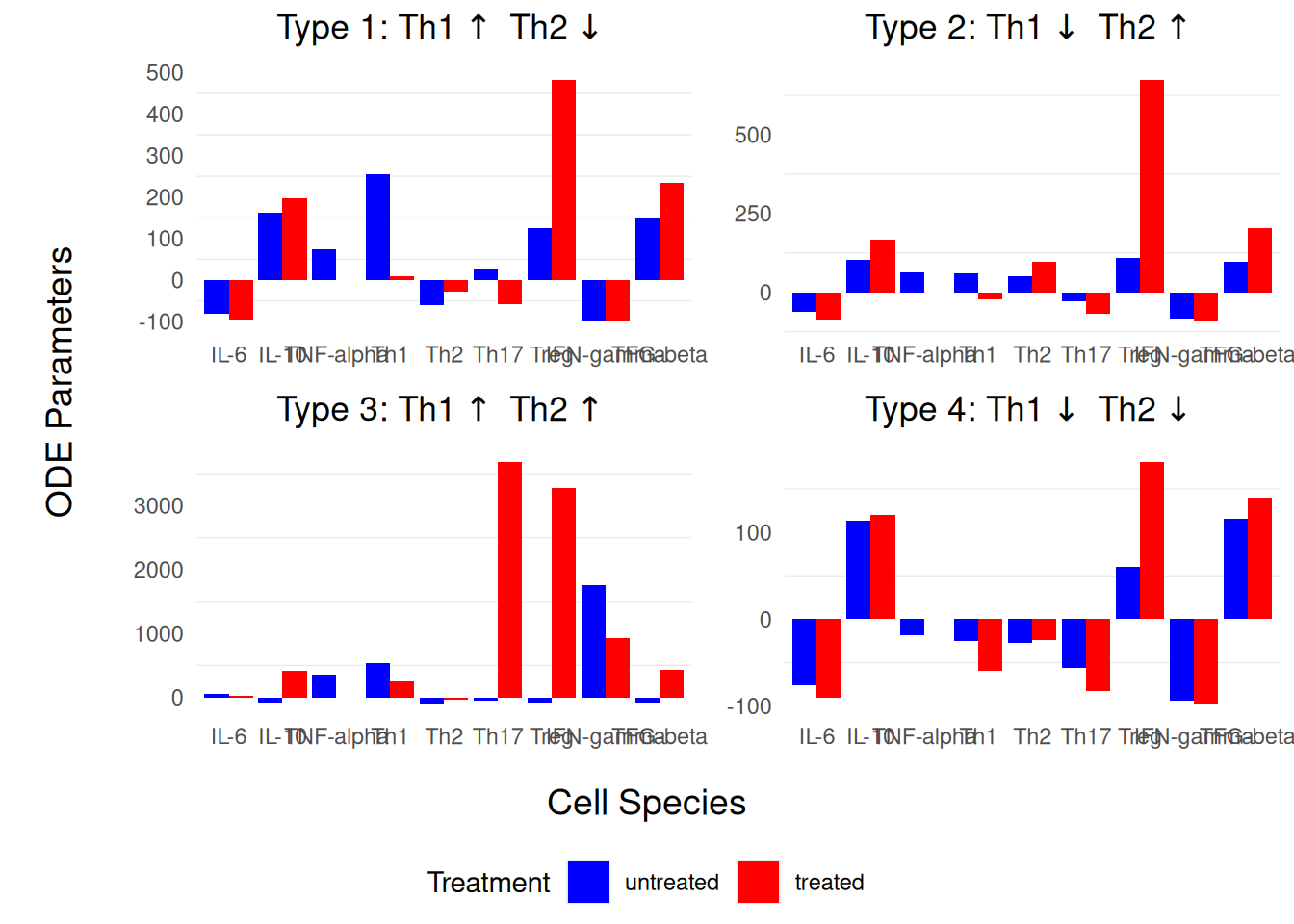
note the final split() instruction: indeed, the expected input is a list of experiences, each element of the list matching a subgroup of patients with their own set of free parameters↩︎
In contrast with documentation, this step seems mandatory, as the output returned by `` has a placeholder typical syntax.↩︎
Webshot table ↩︎

--- title: "Patient stratification" --- The list of packages required for reproducing the analyses on this script are listed in @lst-setup-patient-stratification. Besides, the downloadable R script file [`utils`](../../scripts/utils.R) stores two helper functions: - `get_legend_temp` is a temporary fix to retrieve the legend of any `ggplot2` or `grob` object (used for further customisation of a panel of subplots). For further details on this custom fix, report to [Open `Cowplot` Issue for shared legend feature](https://github.com/wilkelab/cowplot/issues/202). - `colourer` is a custom styling function displaying all positive values as *red*, and negative ones as *blue* (used with `flextable`). ```{r} #| label: setup-stratif #| lst-label: lst-setup-patient-stratification #| lst-cap: Packages required for analysing biological differences between patient conditions. library(CoRC) # Data wrangling library(dplyr) library(readr) # Table visualisation library(scales) library(flextable) # Plot visualisation library(ggplot2) library(latex2exp) library(cowplot) source("../../scripts/utils.R") ``` ## Parameter estimation and patient stratification To run an experimental design, we need: - the model itself, and notably the steady-state concentrations, and the parameter constants. - Experimental data, where for a given condition (here, patient cluster), the columns correspond to the species concentrations, and the rows to the indiviudal observations. Real-life measures of fold changes have been reported in @tbl-experiment-data. - The R code used for loading the healthy model and the clinical datasets, is reported in @lst-load-experiences^[note the final `split()` instruction: indeed, the expected input is a list of experiences, each element of the list matching a subgroup of patients with their own set of free parameters]. ### Differential analyses **Note that @lo2016po did not provide unfortunately the individual cytokine concentrations, preventing from reproducing the differential analyses and quite hampering the validity of [Parameter estimation](https://copasi.org/Support/User_Manual/Tasks/Parameter_Estimation/) Task.** ```{r} #| lst-label: lst-load-experiences #| label: load-healthy #| lst-cap: Code snippet not run, used for illustration example. # Load Healthy ODE model along with the parameter constants healthy_model <- loadModel("../../models/team_2016_final_model_lo2016_2025_05_13.cps") healthy_steaty_state <- runSteadyState( calculate_jacobian = FALSE, model = healthy_model )$species |> dplyr::select(name, concentrationH = concentration) # Load experimental datasets providing real-life concentrations of cytokines cluster_type <- c("Type 1", "Type 2", "Type 3", "Type 4") data_experiment <- readr::read_csv("../../data/IBD DGEA.csv", show_col_types = FALSE) |> tidyr::pivot_longer(!cluster, names_to = "name", values_to = "concentration") |> dplyr::left_join(healthy_steaty_state, by = "name") |> mutate( concentration = if_else(!is.na(concentrationH), concentrationH * (1 + concentration / 100), concentration ), concentrationH = NULL ) |> tidyr::pivot_wider(names_from = name, values_from = concentration) |> split(f = cluster_type) ``` ```{r} #| label: tbl-experiment-data #| echo: false #| tbl-cap: Fold changes of *cytokine* concentrations obtained from clinical data, reported in *Table 7*, [@lo2016po, pp. 13]. `Species` is the cytokines' name, while cluster indicator is returned by `Types of disease`. Note that we have not reported species concentrations of $T-Bet$, $Gata3$, $ROR \gamma t$, and $Foxp3$ as not measured in the ODE model. data_experiment_displayed <- readr::read_csv("../../data/IBD DGEA.csv", show_col_types = FALSE) |> tidyr::pivot_longer(!cluster, names_to = "name", values_to = "concentration") |> dplyr::inner_join(healthy_steaty_state, by = "name") |> mutate(`fold change`= concentration, concentration = concentrationH * (1 + concentration / 100), concentrationH = formatC(concentrationH, format = "e", digits = 2), concentration = formatC(concentration, format = "e", digits = 2)) |> relocate(concentrationH, .before = concentration) labels <- list( name = "Species", cluster = "Types of disease", concentrationH = "Species' concentration at steady-state", concentration = "Concentrations in IBD clusters") flextable(data_experiment_displayed) |> colformat_double(j = c("fold change"), suffix ="%") |> set_header_labels(values = labels) |> footnote(j = "name", i = c(4, 5, 9, 10, 14, 15, 19, 20), value = as_paragraph("These quantities have not been measured, but rather estimated from the model."), part = "body", ref_symbols = c("*")) |> set_caption("Table 7: Fold changes of the cytokine and T cell concentrations obtained from clinical data.") ``` ### Configure the experimental design and the numerical optimisations ```{r} #| label: define-experiences #| # define the free parameters ---- # define larger lower and upper bounds free_parameters_key <- getParameters(c( "(Prod of Ig from T1).k1", "(Prod of Ia from T1).k1", "(Prod of Ib from Tr).k1", "(Prod of I10 from Tr).v10r", "(Induction of T1 from M).s12", "(Induction of T2).s4", "(Induction of T17).s21", "(Induction of T17).s6", "(Induction of Tr).sb", "(Induction of Tr).s10" ), model = healthy_model)$key fit_parameters <- purrr::map(free_parameters_key, function(param) { val <- getParameters(param)$value defineParameterEstimationParameter( ref = parameter(param, "Value"), start_value = val, lower_bound = 1e-15, upper_bound = 1e4 ) }) mapping_present <- getSpeciesReferences( key = c("I6", "I10", "Ia", "Ib", "Ig"), model = healthy_model ) |> pull(concentration) fit_experiments <- purrr::map(data_experiment, ~ defineExperiments( experiment_type = "steady_state", data = .x, types = c( "ignore", "dependent", "dependent", "dependent", "ignore", "ignore", "ignore", "ignore", "ignore", "ignore" ), mappings = c(NA, mapping_present, rep(NA, 4)), weight_method = "mean_square" )) ``` ```r free_parameters_key <- getParameters(c("(Prod of Ig from T1).k1", # <1> "(Prod of Ia from T1).k1", # <1> "(Prod of Ib from Tr).k1", # <1> "(Prod of I10 from Tr).v10r", # <1> "(Induction of T1 from M).s12", # <1> "(Induction of T2).s4", # <1> "(Induction of T17).s21", # <1> "(Induction of T17).s6", # <1> "(Induction of Tr).sb", # <1> "(Induction of Tr).s10"), model = healthy_model)$key # <1> fit_parameters <- purrr::map(free_parameters_key, function(param) { # <2> val <- getParameters(param)$value # <2> defineParameterEstimationParameter( # <2> ref = parameter(param, "Value"), # <2> start_value = val, # <2> lower_bound = 1e-15, # <2> upper_bound = 1e4) # <2> }) # <2> mapping_present <- getSpeciesReferences( key = c("I6", "I10", "Ia", "Ib", "Ig"), model = healthy_model ) |> pull(concentration) fit_experiments <- purrr::map(data_experiment, ~ defineExperiments( # <3> experiment_type = "steady_state", # <3> data = .x, # <3> types = c( # <3> "ignore", "dependent", "dependent", "dependent", # <3> "ignore", "ignore", "ignore", "ignore", "ignore", "ignore"), # <3> mappings = c(NA, mapping_present, rep(NA, 4)), # <4> weight_method = "mean_square" # <5> )) # <3> ``` 1. To adjust the variations of steady-state concentrations observed in the identified four subgroups of patients suffering from Inflammatory Bowel Disease, @lo2016po chose to play with 10 biological constants (10 degrees of freedom). Note that for the system of equations to be **determined** (at the very least), the number of free parameters to estimate must be equal or inferior to the number of equations (here, one by species included in the ODE model, aka 15). 2. We initialise the iterative search by initialising the 10 free parameters with the biological constant vitals observed in healthy individuals. Besides, we can enforce bounds (either for each of the parameters, or shared by all of them), coercing the optimisation algorithm not to go beyond. 3. For each of the patient subgroups, we need to provide the type of experiment (either `steady-state`, or `time_course` when several time points have been considered in the design), the measured concentrations diverging from the average concentrations in healthy patients with `data`, define each of the measured variables (constant with `independent`, `dependent` if used for tailoring the parameter estimates, or `ignore` if not quantified in the ODE model). We had only the averaged expression per patient subgroup To better capture within-patient variability, it would have been valuable to provide the individual cytokine profiles, and perform a [**multiple least-squares regression, aka MMR**](https://en.wikipedia.org/wiki/General_linear_model) task. 4. `mappings` guarantees the proper pairing between COPASI variables and string values of column names^[In contrast with documentation, this step seems mandatory, as the output returned by `` has a **placeholder** typical syntax.]. 5. Finally, the [`weight_method`] coupled with `weights` describe for each variable the assumed mean-variation trend. Report to COPASI Manual, section [*Experimental Data*](https://copasi.org/Support/User_Manual/Tasks/Parameter_Estimation/Experimental_Data/), for further details. Finally, once the experimental design and optimisation criteria have been configured independently for each free parameter and patient subgroup, we have to run the parameter estimation itself: ```{r} #| label: runParameterEstimation #| collapse: true #| cache: false absolute_parameter_per_cluster <- purrr::map(fit_experiments, function(cluster) { # CoRC update imposes to restart from a clean model for parameter estimation CoRC::clearParameterEstimationParameters(model = healthy_model) CoRC::clearExperiments(model = healthy_model) return(runParameterEstimation( parameters = fit_parameters, experiments = cluster, method = list( method = "LevenbergMarquardt", log_verbosity = 0, iteration_limit = 200, tolerance = 1e-5 ), update_model = FALSE, randomize_start_values = FALSE, create_parameter_sets = TRUE, calculate_statistics = FALSE, model = healthy_model )$parameters) }) # Make results directly comparable with Table 8 by switching from absolute to relative ratios relative_parameter_per_cluster <- absolute_parameter_per_cluster |> purrr::list_rbind(names_to = "cluster") |> dplyr::select(cluster, parameter, start_value, value) |> mutate (relative_concentration = 100*(value - start_value)/start_value, start_value = NULL, value = NULL) |> tidyr::pivot_wider(names_from = parameter, values_from = relative_concentration) ``` ```r absolute_parameter_per_cluster <- purrr::map(fit_experiments, function(cluster) { # <1> CoRC::clearParameterEstimationParameters(model = healthy_model) # <2> CoRC::clearExperiments(model = healthy_model) # <2> return(runParameterEstimation( # <3> parameters = fit_parameters, # <3> experiments = cluster, # <3> method = list(method = "LevenbergMarquardt", # <4> iteration_limit = 500, # <4> tolerance = 1e-6), # <4> update_model = FALSE, # <3> randomize_start_values = FALSE, # <3> create_parameter_sets = TRUE, # <3> calculate_statistics = FALSE, # <3> model = healthy_model # <3> )$parameters) }) ``` 1. We learn a configuration of 10 free parameters independently for each patient subgroup. 2. Recall that in COPASI, models are modified by reference rather than by copy. These auxiliary functions, `clearParameterEstimationParameters` and `clearExperiments` guarantee a fresh start for parameter estimation for each scenario. 3. The core function, `runParameterEstimation`, of the pipeline for estimating varying constants across distinct biological conditions. 4. There are plenty of optimisation approaches to reduce the discrepancy between the healthy-state concentrations of immune cells, and the ones observed across each patient cluster, listed in [Optimization Methods](https://copasi.org/Support/User_Manual/Methods/Optimization_Methods/). **Unfortunately, the precise optimisation method used in @lo2016po has not been detailed, nor the hyperparameters used.** We arbitrarily chose the [Levenberg - Marquardt](https://copasi.org/Support/User_Manual/Methods/Optimization_Methods/Levenberg_-_Marquardt/) approach that is a good compromise between first-order, steepest descent approaches, and second-order, Newton-Raphson like approaches (see @tip-optimisation for details). The `iteration_limit` determines the maximum number of iterations the algorithm shall perform, while `tolerance` is the numerical precision to reach between two consecutive iterations. ::: {#tip-optimisation .callout-tip title="Optimisation Descent Methods" collapse="true"} Consider a multivariate function $f(\mathbf{x})$ that we want to **maximize** with respect to $\mathbf{x}$ (for instance, we may want to minimise the mean-squared error between estimated steady-state concentrations and ones measured in each patient subgroup). Standard unconstrained optimization approaches include *Gradient Descent* (see [@eq-GD]), *Newton-Raphson* (see [@eq-NR]) and *Levenbergh-Marquart* (see [@eq-LM]): --- The **Steepest Descent Approach**, where the method updates $\mathbf{x}$ in the direction of the gradient (steepest slope): $$ \mathbf{x}_{k+1} = \mathbf{x}_k + \alpha_k \nabla f(\mathbf{x}_k) $${#eq-GD} where: - $\nabla f(\mathbf{x}_k)$ is the gradient of $f$ at $\mathbf{x}_k$, - $\alpha_k$ is the **step size (learning rate)**, sometimes fixed. Playing on this parameter may prevent revolving round the optimum. - **The steepest descent method only converges linearly, but is guaranteed to converge.** --- The **Newton-Raphson Approach** is a second-order method, requiring the computation of the *Hessian matrix*: $$ \mathbf{x}_{k+1} = \mathbf{x}_k + \mathbf{H}^{-1}(\mathbf{x}_k) \nabla f(\mathbf{x}_k) $${#eq-NR} where: - $\mathbf{H}(\mathbf{x}_k) = \nabla^2 f(\mathbf{x}_k)$ is the Hessian matrix, - $\nabla f(\mathbf{x}_k)$ is the gradient. **On the other hand, the Newton method converges quadratically towards the minimum in its vicinity. However, it's really sensible to the initialisation, and may not converge at all if it is far away from it**. --- The **Levenberg-Marquardt Descent Approach** (@eq-LM): $$ \mathbf{x}_{k+1} = \mathbf{x}_k + \left( \mathbf{H}(\mathbf{x}_k) + \lambda \mathbf{I} \right)^{-1} \nabla f(\mathbf{x}_k) $${#eq-LM} where $\lambda$ is a dampening hyper-parameter controlling the trade-off between gradient descent, when $\lambda \to \infty$, and Newton’s method $\lambda \to 0$. ::: ### Reporting of parameter estimations{#sec-parameter-estimation} Our estimations are compared with *Table 8*, [@lo2016po, pp. 13] variations in @tbl-parameter-estimation. **Of note, all tables in the original paper were provided as screenshots and images, rather than CSV files, preventing straightforward reproducibility of the results**. ```{r} #| label: tbl-parameter-estimation #| echo: true #| tbl-cap: Estimation of parameter variations in different patient subgroups, reported in *Table 8*, [@lo2016po, pp. 13]^[[Webshot table](https://doi.org/10.1371/journal.pone.0165782.t008)]. # flextable formatting and variables variable_labels <- list( cluster = "Type of diseases", `(Prod of Ig from T1).k1` = "coefficient of IFN-gamma by Th1", `(Prod of Ia from T1).k1` = "coefficient of TNF-alpha by Th1", `(Prod of Ib from Tr).k1` = "coefficient of TGF-beta by Treg", `(Prod of I10 from Tr).v10r` = "coefficient of IL-10 by Treg", `(Induction of T1 from M).s12` = "activation of Th1 cells", `(Induction of T2).s4` = "activation of Th2 cells", `(Induction of T17).s21` = "activation of Th17 cells", `(Induction of T17).s6` = "activation of Th17 cells", `(Induction of Tr).sb` = "activation of Treg cells", `(Induction of Tr).s10` = "activation of Treg cells" ) header_row <- c( "\\text{Type of diseases}", "\\nu_{\\gamma_1}", "\\nu_{\\alpha_1}", "\\nu_{\\beta_{\\rho}}", "\\nu_{10_{\\rho}}", "\\sigma_{12}", "\\sigma_{4}", "\\sigma_{21}", "\\sigma_{6}", "\\sigma_{\\beta}", "\\sigma_{10}") |> as_equation() |> as_paragraph() # flextable generation relative_parameter_variations_flextable <- flextable(relative_parameter_per_cluster) |> # Add gradient colouring based on values bg( j = setdiff(names(variable_labels), "cluster"), bg = colourer) |> # Format numbers (optional for consistent display) colformat_double(j = setdiff(names(variable_labels), "cluster"), suffix = "%", big.mark = ",", digits = 1) |> append_chunks(j = "cluster", # what to append as_equation(c("\\text{Th1}\\uparrow \\text{Th2}\\downarrow", "\\text{Th1}\\downarrow \\text{Th2}\\uparrow", "\\text{Th1}\\uparrow \\text{Th2}\\uparrow", "\\text{Th1}\\downarrow \\text{Th2}\\downarrow")) ) |> # Rename columns using LaTeX-like notation set_header_labels(values = variable_labels ) |> add_header_row(values = header_row, colwidths = rep(1, 11), top = FALSE ) |> align(align = "center", part = "all") |> set_caption("Table 8: Parameter variations in different types of diseases. In blue, disease subtype induces shrinkage of the coefficients, while red values correspond to increased parameter uptakes. ") |> merge_at(part = "head", i = 1:2, j = 1) relative_parameter_variations_flextable ``` One of the major advantages of `flextable` lies in its ability to save the generated flextable object in a variety of formats, including `docx`, and `html`, as illustrated in @lst-flextable-output (or even several ones simultaneously). ```{r} #| label: flextable-output #| eval: false #| lst-label: lst-flextable-output #| lst-cap: Flextable multiple outputs. save_as_html(relative_parameter_variations_flextable, path = "../../results/Table8.html", title = "Table 8: Parameter variations per disease subtype." ) save_as_docx(relative_parameter_variations_flextable, path = "../../results/Table8.docx", title = "Table 8: Parameter variations per disease subtype." ) ``` ## Treatment outcome and patient stratification The objective of this section is to predict the efficiency of a novel anti-TNF-$\alpha$ treatment, assuming that the blocking treatment is equivalent to force the concentration of TNF-$\alpha$ to remain zero, and calculate the change of other variables at the **steady-state concentrations**. Second objective is to determine the efficiency of the treatment conditioned to the *patient endotype* determined using *patient stratification* approaches. ### Load Free Parameter variations in different types of diseases **Since the results of parameter estimation reported in @sec-parameter-estimation differ significantly from the results reported in the original paper, *Table 8*, [@lo2016po, pp. 13](https://journals.plos.org/plosone/article/figure?id=10.1371/journal.pone.0165782.t008), we directly retrieve in that section the original estimates from @lo2016po**. ```{r} #| label: load-parameter-variations #| collapse: true ## Prepare parameter variations for each of the four patient subtypes ---- healthy_model <- suppressWarnings(loadModel("../../models/team_2016_final_model_lo2016_2025_05_13.cps")) # retrieve parameter mapping parameters_per_clusters <- getParameters(c("(Prod of Ig from T1).k1", "(Prod of Ia from T1).k1", "(Prod of Ib from Tr).k1", "(Prod of I10 from Tr).v10r", "(Induction of T1 from M).s12", "(Induction of T2).s4", "(Induction of T17).s21", "(Induction of T17).s6", "(Induction of Tr).sb", "(Induction of Tr).s10"), model = healthy_model) # retrieve parameter variations specific to each disease subtype ... patient_group <- c("Type1", "Type2", "Type3", "Type4") parameters_per_clusters <- parameters_per_clusters |> dplyr::inner_join(readr::read_csv("../../data/IBD subgroups.csv", show_col_types = FALSE), by = "key") |> rename(healthy = value) |> dplyr::select(-mapping) |> # ... and convert relative ratios to absolute dplyr::mutate(across(all_of(patient_group), \(x) healthy * (1 + x/100))) # run healthy steady state healthy_steaty_state <- runSteadyState( calculate_jacobian = FALSE, model = healthy_model)$species |> dplyr::select(name, concentrationH = concentration) |> filter (name %in% c("I6", "I10", "Ia", "T1", "T2","T17", "Tr", "Ig", "Ib")) ``` ### Model the effect of TNF-alpha blockade ```{r} #| label: model-tnf-blockade #| echo: false # Infer steady states for each patient subgroup, with and without anti-TNF-alpha treatment ---- steady_states_per_cluster <- purrr::map(patient_group, function(cluster) { disease_model_without_treatment <- healthy_model |> saveModelToString() |> loadModelFromString() setParameters(model = disease_model_without_treatment, key = parameters_per_clusters$key, value = parameters_per_clusters[[cluster]]) # without anti-TNF alpha treatment without_treatment_steady_state <- runSteadyState( calculate_jacobian = FALSE, model = disease_model_without_treatment)$species |> dplyr::select(name, concentration) |> inner_join(healthy_steaty_state, by = "name") |> mutate (concentration = 100* (concentration - concentrationH) / concentrationH) |> dplyr::select(-concentrationH) |> mutate(cluster = cluster, category = "untreated") # with anti-TNF alpha treatment disease_model_with_treatment <- suppressWarnings(disease_model_without_treatment |> saveModelToString() |> loadModelFromString()) # to that end, coerce TNF-alpha to remain fixed and null throughout the whole process setSpecies( key = "Ia{compartment}", initial_concentration = 0, type ="fixed", model = disease_model_with_treatment ) with_treatment_steady_state <- runSteadyState( calculate_jacobian = FALSE, model = disease_model_with_treatment)$species |> dplyr::select(name, concentration) |> inner_join(healthy_steaty_state, by = "name") |> mutate (concentration = 100* (concentration - concentrationH) / concentrationH) |> dplyr::select(-concentrationH) |> tibble::add_row(name = "Ia", concentration = 0) |> mutate(cluster = cluster, category = "treated") return (rbind(without_treatment_steady_state, with_treatment_steady_state)) }) |> dplyr::bind_rows() ``` ```r steady_states_per_cluster <- purrr::map(patient_group, function(cluster) { # without anti-TNF alpha treatment disease_model_without_treatment <- healthy_model |> saveModelToString() |> loadModelFromString() # <1> setParameters(model = disease_model_without_treatment, # <1> key = parameters_per_clusters$key, # <1> value = parameters_per_clusters[[cluster]]) # <1> without_treatment_steady_state <- runSteadyState( # <1> calculate_jacobian = FALSE, # <1> model = disease_model_without_treatment)$species |> # <1> dplyr::select(name, concentration) |> # <1> inner_join(healthy_steaty_state, by = "name") |> # <1> mutate (concentration = 100* (concentration - concentrationH) / concentrationH) |> # <1> dplyr::select(-concentrationH) |> # <1> mutate(cluster = cluster, category = "untreated") # <1> # with anti-TNF alpha treatment disease_model_with_treatment <- suppressWarnings(disease_model_without_treatment |> saveModelToString() |> loadModelFromString()) setSpecies(key = "Ia{compartment}", # <2> initial_concentration = 0, # <2> type ="fixed", # <2> model = disease_model_with_treatment) # <2> with_treatment_steady_state <- runSteadyState( # <3> calculate_jacobian = FALSE, # <3> model = disease_model_with_treatment)$species |> # <3> dplyr::select(name, concentration) |> # <3> inner_join(healthy_steaty_state, by = "name") |> # <3> mutate (concentration = 100* (concentration - concentrationH) / concentrationH) |> # <3> dplyr::select(-concentrationH) |> # <3> tibble::add_row(name = "Ia", concentration = 0) |> # <3> mutate(cluster = cluster, category = "treated") # <3> return (rbind(without_treatment_steady_state, with_treatment_steady_state)) }) |> dplyr::bind_rows() # <4> ``` 1. Estimate *steady-state* conditions for each of the four patient subgroups identified, without anti-TNF-$\alpha$ treatment. 2. Constrain TNF-$\alpha$ to remain `fixed` and **null** by setting the initial concentration level to $0$. **Both parameters are required** to ensure absence of TNF-$\alpha$. 3. Predict the new *steady-state* conditions after therapeutic treatment. 4. `dplyr::bind_rows()` merges a list of `data.frame` into a single one. ### Simulation visualisations of the fold changes of the cytokine and T cell concentrations We have reproduced *Fig.3* from @lo2016po, pp. 13, in @fig-treatment-blockade, using a combination of `ggplot2`for individual barplot representations and `cowplot` for individual 'ggplot' concatenations. ```{r} #| collapse: true #| label: fig-treatment-blockade #| fig-cap: Simulation results of the **fold changes** of the cytokine and T-cell concentrations when TNF-$\alpha$ is completely blocked in the four group of identified patients. Blue bars represent the results of pre-treatment; red bars represent the results of post-treatment with TNF-$\alpha$ blockage. Reproduction of [@lo2016po, pp. 13], Fig.3. # Reproduce boxplots of Figure 3, pre and post-treatment ---- # Format dataset for plotting steady_states_per_cluster_plot <- steady_states_per_cluster |> mutate (name = factor (name, levels = c("I6", "I10", "Ia", "T1", "T2", "T17", "Tr", "Ig", "Ib"), labels = c("IL-6", "IL-10", "TNF-alpha", "Th1", "Th2", "Th17", "Treg", "IFN-gamma", "TFG-beta"), ordered = TRUE), category = factor(category, levels = c("untreated", "treated"), ordered = TRUE)) cluster_labels <- c("Type 1: Th1\\uparrow Th2\\downarrow", "Type 2: Th1\\downarrow Th2\\uparrow", "Type 3: Th1\\uparrow Th2\\uparrow", "Type 4: Th1\\downarrow Th2\\downarrow") names(cluster_labels) <- c("Type1", "Type2", "Type3", "Type4") ### Retrieve legend ---- global_plot <- ggplot(data = steady_states_per_cluster_plot, mapping = aes(x = name, y = concentration, fill = category)) + geom_col(position = "dodge") + scale_fill_manual(name ="Treatment", values=c("blue", "red")) + guides(color = guide_legend(nrow = 1)) + theme(legend.position = "bottom") ### Generate bar plot for each disease subtype ---- list_plots <- purrr::imap(cluster_labels, ~ ggplot(data = steady_states_per_cluster_plot |> filter(cluster==.y), mapping = aes(x = name, y = concentration, fill = category)) + geom_col(position = "dodge")+ labs(x = NULL, y = NULL) + scale_fill_manual(name ="Treatment", values=c("blue", "red")) + theme_minimal() + theme(panel.grid.major = element_blank(), legend.position = "none", plot.title = element_text(hjust = 0.5)) + ggtitle(TeX(.x))) ### Combine barplots into a 2x2 grid ---- plot_grid_combined <- cowplot::plot_grid(plotlist = list_plots, ncol = 2, align = "hv", axis = "tblr") x_label <- ggdraw() + draw_label("Cell Species", x = 0.5, y = 0.5) y_label <- ggdraw() + draw_label("ODE Parameters", x = 0.5, y = 0.5, angle = 90) # Add global y label plot_grid_combined <- cowplot::plot_grid(y_label, plot_grid_combined, nrow = 1, rel_widths = c(0.1, 1) # Adjust width for the legend ) legend_plot <- get_legend_temp(global_plot) # Add global x label plot_grid_combined <- cowplot::plot_grid(plot_grid_combined, x_label, legend_plot, nrow = 2, ncol =1, rel_heights = c(1, 0.1) # Adjust width for the legend ) plot_grid_combined <- cowplot::plot_grid( plot_grid_combined, legend_plot, nrow = 2, rel_heights = c(1, 0.1) # Adjust width for the legend ) plot_grid_combined ```