5.1 Deconvolution with reference distributions: a review of methods that use more than the mean

Bastien Chassagnol

2026-11-02

Scope

First-generation deconvolution fits a bulk profile with the mean expression of each purified population. This review covers the methods that also use the distribution of the purified profiles: at least their variance, and in some cases a covariance between genes or between cell types. DeCovarT belongs to that family: it plugs in a gene–gene covariance per cell type and maximises a Gaussian-convolution likelihood (population generative vignette).

Every method is read through the same lens: what its observation law implies about the measurement process, most often UMI counts from single cells. Sec. 1 states the measurement and expression models that lens relies on. Sec. 2.2 states the errors-in-variables problem that every method solves, Sec. 2.3 orders the methods on a ladder of noise models, and Sec. 2.4 separates marginal from conditional multivariate models. The methods follow, grouped by what they estimate and what they assume known:

1. reference-based estimation of the composition, split by whether genes are treated as independent (Sec. 2);
2. cell-type-specific moments when the composition is known (Sec. 3);
3. Bayesian reference-based methods, for profiles or for proportions (Sec. 4);
4. semi-reference methods that infer one unknown component (Sec. 5);
5. reference-free methods that use co-expression structure (Sec. 6).

Sec. 7 compares them and lists their caveats. The DeCovarT model rebuilt for single-cell references is in the single-cell generative vignette.

%%{init: {"theme": "sandstone", "flowchart": {"curve": "basis"}}}%%
flowchart TD
  root["Reference distribution used beyond the mean"]
  root --> ref["Reference-based, composition estimated"]
  root --> cts["Composition known, profiles estimated"]
  root --> bay["Bayesian reference-based"]
  root --> semi["Semi-reference: one unknown component"]
  root --> free["Reference-free"]
  ref --> uni["Genes independent: MuSiC, SCDC, RNA-Sieve, DWLS, deMixSC, Bisque, RCTD, DeconV, ReDeconv"]
  ref --> multi["Gene-gene covariance: DECALS, MEAD, DeCovarT"]
  cts --> csnet["CSNet, Unico, imply"]
  bay --> bcts["Profiles: bMIND, EPIC-unmix, BLADE, BEDwARS, BayesPrism, BLEND"]
  bay --> bprop["Proportions: DSection, gnSPADE"]
  semi --> dem["DeMix, DeMixT, DeMixNB, BayICE, ISOpureR"]
  free --> nmf["DSSC, GSNMF+, swCAM"]

Figure 1: Deconvolution methods that use more than the reference mean, grouped by what is known and what is estimated. Colours are not used; the grouping is the one of the sections of this review.

Notation (shared by all vignettes; aligned with the article)

Gene g=1,\ldots,G; cell type j=1,\ldots,J (a second type is \ell); bulk sample i=1,\ldots,N; reference donor (replicate) r=1,\ldots,R; cell c, with C_j reference cells of type j. The index i is dropped inside a derivation and restored in the model statements.

Symbol	Meaning
y_{gi}, \boldsymbol{y}_{\cdot i}	Bulk expression on a linear scale
m_{ji}, n_i=\sum_jm_{ji}	Cells of type j in bulk sample i, and their total
\tilde{\boldsymbol{y}}_{\cdot i}=\boldsymbol{y}_{\cdot i}/n_i	Bulk expression per cell
\boldsymbol{p}_{\cdot i}\in\Delta^{J-1}	Cell fractions, p_{ji}=m_{ji}/n_i
\boldsymbol{\rho}_{i}\in\mathbb{R}^{J-1}	Isometric log-ratio (ILR) coordinates of \boldsymbol{p}_{\cdot i}, \boldsymbol{p}_{\cdot i}=\operatorname{softmax}(\mathbf{V}\boldsymbol{\rho}_i) with a Helmert basis \mathbf{V}
\boldsymbol{q}_{\cdot i}	Transcript fractions, q_{ji}=p_{ji}S_j/\sum_\ell p_{\ell i}S_\ell
\boldsymbol{\mu}_{\cdot j}, \boldsymbol{\Sigma}_j	Mean and G\times G gene–gene covariance of a type-j population profile
\boldsymbol{\Omega}_j=\boldsymbol{\Sigma}_j^{-1}	Precision matrix of type j
\boldsymbol{\Gamma}_g	J\times J covariance across cell types for gene g (bMIND, EPIC-unmix, Unico)
\boldsymbol{x}_{\cdot j,i}	Purified profile of type j in sample i
x_{gc}, \boldsymbol{x}_{\cdot c}, s_c	Raw UMI count of gene g in reference cell c, and the size factor of cell c
\boldsymbol{\lambda}_{\cdot c}, \boldsymbol{z}_{\cdot c}	Size-free expression of cell c; its latent log-expression in the Poisson log-normal (PLN) model
\tilde{\boldsymbol{\mu}}_{\cdot j}=C_j^{-1}\sum_{c\in j}\boldsymbol{x}_{\cdot c}=S_j\boldsymbol{\theta}_{\cdot j}	Per-cell mean of the raw UMI counts of the C_j reference cells of type j
\boldsymbol{\theta}_{\cdot j}, S_j=\mathbf{1}^{\top}\tilde{\boldsymbol{\mu}}_{\cdot j}	Relative abundance (\mathbf{1}^{\top}\boldsymbol{\theta}_{\cdot j}=1) and mean transcriptome size of a type-j cell
\boldsymbol{\Sigma}_{W,j}, \boldsymbol{\Sigma}_{B,j}	Within-donor cell-to-cell covariance of type j (one single-cell sample); between-donor covariance of type j (needs R\ge2 donors)
\boldsymbol{S}_W(\boldsymbol{v})=\sum_jv_j\boldsymbol{\Sigma}_{W,j}, \boldsymbol{S}_B(\boldsymbol{v})=\sum_jv_j^2\boldsymbol{\Sigma}_{B,j}	Linear and quadratic covariance mixtures with weights \boldsymbol{v}
\boldsymbol{V}_j	Empirical covariance of type j, computed from its reference profiles or cells
\boldsymbol{R}_j	Empirical correlation matrix of type j (bold; the scalar R is the number of donors)
\boldsymbol{\Delta}_j=\operatorname{diag}(\boldsymbol{V}_j)	Diagonal matrix of the empirical variances of type j
\lambda	Penalty of a regularised covariance or precision estimator
\psi_g, \mathcal{D}_g	Negative binomial dispersion of gene g; deviance of gene g in a count model
\delta_{gj}	Detection rate of gene g in type j (fraction of cells with a non-zero count)
\varpi_{\ell\mid j}, \varpi_{j\ell}, \bar\varpi	MixSim overlap: probability of misclassifying a draw of j into \ell, pairwise overlap \varpi_{j\ell}=\varpi_{\ell\mid j}+\varpi_{j\mid\ell}, and its average over pairs (BarOmega)
\boldsymbol{T}_{ji}=\sum_{c=1}^{m_{ji}}\boldsymbol{X}_{jic}	Total expression contributed by type j to sample i
a_i	Sample-wide scale between the reference and the bulk library
c_i=a_in_i, \phi_i=a_i^2n_i	Mean scale and variance scale of the single-cell model
b_g, \tilde b_g=b_g^{\mathrm{bulk}}/b_g^{\mathrm{ref}}	Capture efficiency of gene g in one protocol, and the gene-wise platform ratio; \tilde{\boldsymbol{B}}=\operatorname{diag}(\tilde{\boldsymbol{b}})
\boldsymbol{D}_i	Diagonal, heteroscedastic bulk measurement noise

A tilde marks a quantity rescaled to a reference unit: per cell (\tilde{\boldsymbol{y}}, \tilde{\boldsymbol{\mu}}) or relative to the reference protocol (\tilde{\boldsymbol{b}}). \boldsymbol{\Sigma}_j couples genes within one cell type; \boldsymbol{\Gamma}_g couples cell types within one gene. A symbol absent from this table is defined in the vignette that uses it, with one meaning there.

Equations quoted from a paper are translated into these indices; only Table 2 keeps each paper’s own symbols.

Measurement and expression models for single-cell counts

A reference profile is a moment of a latent biological quantity, but it is estimated from counts produced by a sampling protocol. Sarkar and Stephens separate the two: a measurement model p(\boldsymbol{x}\mid\boldsymbol{\lambda}) describes the protocol given the true expression, an expression model p(\boldsymbol{\lambda}) describes the biology, and the observation model p(\boldsymbol{x}) is their composition (Sarkar and Stephens 2021). Fang and Pachter add that the cell-level scale factor is itself a product of a biological and a technical term (Fang and Pachter 2025). Both papers index genes by j and cells by i; below, gene is g and cell is c, so that j remains the cell type.

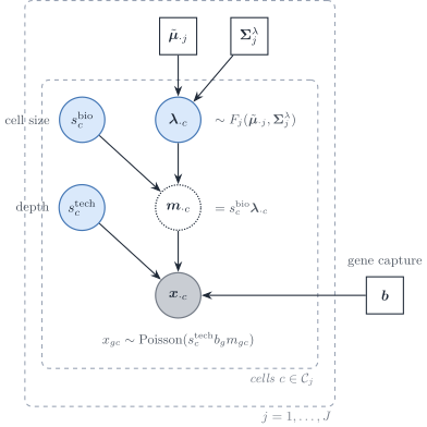
Figure 2: Measurement and expression model of a single-cell reference, in the notation of this vignette. Inside cell type j, the size-free expression \boldsymbol{\lambda}_{\cdot c} follows an expression model F_j with mean \tilde{\boldsymbol{\mu}}_{\cdot j} and covariance \boldsymbol{\Sigma}^{\lambda}_j; the biological size factor turns it into a molecule content; the technical size factor and the gene capture efficiency \boldsymbol{b} act through a Poisson measurement.

Poisson measurement of UMI counts

If each molecule of cell c is captured independently with a small probability, the multivariate hypergeometric sampling of molecules is close to a multinomial and each gene count is Poisson given the true content (Supplementary Note 1 of (Sarkar and Stephens 2021)):

x_{gc}\mid s^{\mathrm{tech}}_c,m_{gc} \sim\mathrm{Poisson}\bigl(s^{\mathrm{tech}}_c\,b_g\,m_{gc}\bigr), \qquad \boldsymbol{m}_{\cdot c}=s^{\mathrm{bio}}_c\,\boldsymbol{\lambda}_{\cdot c}. \tag{1}

Fang and Pachter write the same law as binomial thinning with capture rate b_gs^{\mathrm{tech}}_c, of which the Poisson is the low-capture limit, and normalise \mathbb{E}[s^{\mathrm{bio}}]=\mathbb{E}[s^{\mathrm{tech}}]=1 (their equations 1–2). Sarkar and Stephens instead take the observed library size x_{+c} as the size factor and a relative expression \lambda_{gc}=m_{gc}/m_{+c}; in that convention s^{\mathrm{bio}}_c cancels by construction, which is the removal of biological extrinsic noise that Fang and Pachter warn about. The two conventions are the two directions of the same rank-one Poisson fit: the point-mass MLE \hat\mu_g=\sum_cx_{gc}/\sum_cx_{+c} and the size-factor MLE of Eq. 3 below.

Three remarks connect the protocol to deconvolution.

• UMIs remove most gene-specific distortion. Unique molecular identifiers collapse PCR duplicates, which “substantially reduce unwanted variation, including differences in gene lengths and PCR amplification efficiencies” (Sarkar and Stephens 2021). What remains is a capture efficiency b_g that is constant across cells of one protocol. It is not identified separately from \boldsymbol{\lambda}, and it cancels from every within-protocol contrast, so it is absorbed into \tilde{\boldsymbol{\mu}}_{\cdot j} and \boldsymbol{\Sigma}_{W,j}. It does not cancel between a single-cell reference and a bulk library: the ratio \tilde b_g=b_g^{\mathrm{bulk}}/b_g^{\mathrm{ref}} is the gene-wise platform factor of plug-in scales (Strategy 4). Read-count protocols without UMIs and hybridisation microarrays carry larger gene- and probe-specific factors (amplification, length, affinity), which is why earlier deconvolution methods had to model gene-wise scales explicitly; with UMI references, the gene-wise factor reduces to one cross-platform ratio per gene.
• Random capture biases make the measurement overdispersed; constant ones do not. If b_{gc} varied from cell to cell, the measurement model would be negative binomial rather than Poisson (Box 1 and Supplementary Note 1.2 of Sarkar and Stephens). On spike-in controls the measurement dispersion was below 5\times10^{-3}, which adds about 5% to the variance of a gene with ten observed molecules. Overdispersion seen in single-cell data is therefore an expression property, \boldsymbol{\Sigma}^{\lambda}_j, plus extrinsic noise, not a protocol property.
• Zero inflation belongs to the expression model, if anywhere. Spike-in controls show no zero-generating measurement component, and a point-Gamma expression model beats a Gamma model for only 0.6–8.6% of genes across the datasets tested (Sarkar and Stephens 2021). Zeros are imperfect measurements of small \lambda_{gc} at low depth, “with no need for special terminology or special treatment”. For DeCovarT, which uses only the first two moments of the reference, a zero-inflated observation model is unnecessary: the moments of the counts already contain the zeros. The argument is made for UMI data; the authors note that it may not hold for read counts amplified by PCR without UMIs.

Expression models and the observation models they induce

Integrating the expression model against Eq. 1 gives the observation model gene by gene (Table 1 of (Sarkar and Stephens 2021)).

Table 1: Expression and observation models for UMI counts, after Sarkar and Stephens (Tables 1–2). The measurement model is Poisson throughout.

Expression model for \lambda_{gc}	Observation model for x_{gc}	Examples
Point mass \lambda_{gc}=\mu_g	Poisson	analytic
Gamma, mean \mu_g, variance \mu_g^{2}\phi_g	Negative binomial	edgeR, DESeq2, SAVER
Point-Gamma	Zero-inflated negative binomial	ZINB-WaVE (multigene)
Unimodal or fully nonparametric	Flexible	ashr, DESCEND
Low rank, \lambda_{gc}=\mu_{gc}u_{gc}, \mu=h^{-1}(\boldsymbol{L}\boldsymbol{F}^{\top})	Flexible	GLM-PCA, scVI

A gene whose expression model is a point mass inside a homogeneous population is a Poisson gene: its count has no variability beyond sampling and the extrinsic size factor. Overdispersion relative to a Poisson, the hallmark of the negative binomial, then measures either biological variability of \lambda_{gc} or variability of s_c.

Extrinsic noise, size factors and Poisson genes

Fang and Pachter show that a cell-wide factor explains the baseline overdispersion of single-cell counts. Under Eq. 1 with s_c=s^{\mathrm{bio}}_cs^{\mathrm{tech}}_c independent of \boldsymbol{\lambda}_{\cdot c}, \mathbb{E}[s_c]=1 and \nu=\operatorname{CV}^{2}(s_c), their equation (3) reads, in our notation and inside one cell type,

\frac{\operatorname{Cov}(x_{gc},x_{hc})}{\mathbb{E}[x_{gc}]\mathbb{E}[x_{hc}]} =\nu+(1+\nu)\frac{\Sigma^{\lambda}_{j,gh}}{\tilde\mu_{gj}\tilde\mu_{hj}} +\frac{\delta_{gh}}{\mathbb{E}[x_{gc}]}, \qquad 1+\nu=(1+\nu^{\mathrm{bio}})(1+\nu^{\mathrm{tech}}). \tag{2}

For two genes that are intrinsically uncorrelated, or for one gene that is intrinsically Poisson, the normalised covariance equals \nu (their equation 5). That identity gives an estimator of \nu (the mode of the normalised covariances over gene pairs) and a selection rule for Poisson genes (those whose normalised variance minus the Poisson term has a bootstrap interval containing \hat\nu). On those genes \mathcal{P}, the size factor has the closed-form MLE

\hat s_c=\frac{\sum_{g\in\mathcal{P}}x_{gc}}{\sum_{g\in\mathcal{P}}\tilde\mu_{gj}}. \tag{3}

Two findings matter here. Normalising each cell by its total removes s^{\mathrm{bio}}_c together with s^{\mathrm{tech}}_c, and with it the biological extrinsic variability, including cell size (Fang and Pachter 2025). In peripheral blood, sums over Poisson genes no longer track total UMI counts and differ between cell types, so the choice of size factor changes downstream comparisons. Separating s^{\mathrm{tech}}_c from s^{\mathrm{bio}}_c needs external controls (spike-ins, ambient RNA, pooled RNA); the nascent-mRNA counts did not fit the binomial sampling model in their pooled-RNA experiment.

What the measurement model implies for the reference covariance

Write the same identity in matrix form (a direct consequence of Eq. 1 and the law of total covariance; the derivation is ours). With \boldsymbol{\mathcal{B}}=\operatorname{diag}(\boldsymbol{b}),

\operatorname{Cov}(\boldsymbol{x}_{\cdot c}\mid c\in j) =\underbrace{\operatorname{diag}\bigl(\boldsymbol{\mathcal{B}}\tilde{\boldsymbol{\mu}}_{\cdot j}\bigr)}_{\text{Poisson measurement}} +\boldsymbol{\mathcal{B}}\Bigl[ \underbrace{(1+\nu)\boldsymbol{\Sigma}^{\lambda}_j}_{\text{biology}} +\underbrace{\nu\,\tilde{\boldsymbol{\mu}}_{\cdot j}\tilde{\boldsymbol{\mu}}_{\cdot j}^{\top}}_{\text{size factor}} \Bigr]\boldsymbol{\mathcal{B}}. \tag{4}

The sample covariance of raw UMI counts, which is what a single-cell reference returns as \hat{\boldsymbol{\Sigma}}_{W,j}, mixes three objects. Only part of it belongs in the bulk law.

1. The Poisson diagonal is single-cell measurement noise. It is produced at single-cell depth and is not part of the tissue. A bulk library has its own sampling noise, on its own depth, which a diagonal bulk term would carry. Plugging raw-count covariances into \boldsymbol{S}_W imports the reference sampling noise into the bulk covariance; subtracting \operatorname{diag}(\bar{\boldsymbol{x}}_j) first removes it.
2. The technical size-factor term is not biology either. The rank-one term \nu^{\mathrm{tech}}\tilde{\boldsymbol{\mu}}_{\cdot j}\tilde{\boldsymbol{\mu}}_{\cdot j}^{\top} induces a positive correlation between all genes. It inflates the apparent network and is a protocol artefact.
3. The biological size factor is part of the bulk. Cells of one type differ in volume and cycle phase; a tissue sums those cells as they are. The term \nu^{\mathrm{bio}}\tilde{\boldsymbol{\mu}}_{\cdot j}\tilde{\boldsymbol{\mu}}_{\cdot j}^{\top} belongs in \boldsymbol{\Sigma}_{W,j}, and library-size normalisation that removes it understates the within-type variance that the bulk accumulates.

The corresponding moment estimator, with \hat\nu^{\mathrm{tech}} from spike-ins and \hat\kappa=\hat\nu^{\mathrm{tech}}/(1+\hat\nu^{\mathrm{tech}}), is

\hat{\boldsymbol{\Sigma}}_{W,j} =\boldsymbol{V}_j-\operatorname{diag}(\bar{\boldsymbol{x}}_j) -\hat\kappa\, \Bigl[\boldsymbol{V}_j-\operatorname{diag}(\bar{\boldsymbol{x}}_j)+\bar{\boldsymbol{x}}_j\bar{\boldsymbol{x}}_j^{\top}-\frac{\boldsymbol{V}_j}{C_j}\Bigr], \tag{5}

where \boldsymbol{V}_j is the unbiased sample covariance of the C_j type-j cells and \bar{\boldsymbol{x}}_j their mean. It estimates the s^{\mathrm{tech}}-free covariance of \boldsymbol{\mathcal{B}}\boldsymbol{m}_{\cdot c}, \boldsymbol{\mathcal{B}}[(1+\nu^{\mathrm{bio}})\boldsymbol{\Sigma}^{\lambda}_j+\nu^{\mathrm{bio}}\tilde{\boldsymbol{\mu}}_{\cdot j}\tilde{\boldsymbol{\mu}}_{\cdot j}^{\top}]\boldsymbol{\mathcal{B}}, obtained by solving Eq. 4 with 1+\nu=(1+\nu^{\mathrm{bio}})(1+\nu^{\mathrm{tech}}) (our derivation). Given \nu^{\mathrm{tech}} it is unbiased. The term -\boldsymbol{V}_j/C_j is needed because \bar{\boldsymbol{x}}_j\bar{\boldsymbol{x}}_j^{\top} overestimates the outer product of the means by \operatorname{Cov}(\boldsymbol{x})/C_j; without it the estimator is biased by -\kappa\operatorname{Cov}(\boldsymbol{x})/C_j, which a simulation with C_j=10 cells detects. The error of an estimated \hat\nu^{\mathrm{tech}} is not covered by this statement. Plugging in the total extrinsic noise \nu, which a size factor fitted on Poisson genes estimates (Sec. 1.3), returns \boldsymbol{\mathcal{B}}\boldsymbol{\Sigma}^{\lambda}_j\boldsymbol{\mathcal{B}}: it removes the biological share \nu^{\mathrm{bio}}\boldsymbol{\mathcal{B}}(\boldsymbol{\Sigma}^{\lambda}_j+\tilde{\boldsymbol{\mu}}_{\cdot j}\tilde{\boldsymbol{\mu}}_{\cdot j}^{\top})\boldsymbol{\mathcal{B}} with the technical one. Whether this denoised covariance enters the bulk alone or with the bulk’s own sampling term depends on the bulk depth per cell (raw or denoised). Estimating \nu^{\mathrm{tech}} before the deconvolution is the first plug-in of Strategy 4 (plug-in scales (Strategy 4)).

ComBat, scVI and scANVI: what they remove

Three families of correction are often proposed for the same job. Each removes a different quantity, on a different unit.

• ComBat corrects “both additive and multiplicative batch effects” in an empirical-Bayes framework (Johnson, Li and Rabinovic 2007, as summarised by Zhang 2025, p. 1): a location and a scale per gene and batch, shrunk across genes. Its count version, ComBat-ref, fits \log\mu_{gij}=\alpha_g+\gamma_{gi}+\beta_{g,\mathrm{cond}(j)}+\log N_j for gene g, batch i and sample j with a pooled negative binomial dispersion per batch, keeps the batch of smallest dispersion as reference, sets \log\tilde\mu_{gij}=\log\mu_{gij}+\gamma_{g1}-\gamma_{gi}, and maps each count by matching negative binomial distribution functions, zeros to zeros (Zhang 2025, p. 2). The unit is a bulk sample inside a batch; the biological condition is a term of the model, and single-cell data are left to future work (p. 6).
• scVI draws, for cell n, a latent \boldsymbol{z}_n\sim\mathcal{N}(\boldsymbol{0},\mathbf{I}), a library factor \ell_n\sim\mathrm{LogNormal} whose prior is the empirical mean and variance of the log library size of its batch, frequencies \boldsymbol{\rho}_n=f_w(\boldsymbol{z}_n,s_n) that sum to one over genes, and counts \mathrm{Poisson}(\ell_nw_{ng}) with w_{ng}\sim\mathrm{Gamma}(\rho_{gn},\theta_g), plus zero inflation (Lopez et al. 2018, author manuscript pp. 8–9). \ell_n “represents nuisance variation due to differences in capture efficiency and sequencing depth”, and the batch s_n enters the decoder, so \rho_{ng} is “a batch-corrected, normalized estimate of the percentage of transcripts” (p. 3). Genes are independent given (\boldsymbol{z}_n,\ell_n) (p. 8), so gene–gene covariance passes through the 10-dimensional \boldsymbol{z}_n only (p. 3). No reference is used.
• scANVI adds a cell-type label c_n with a uniform prior, a within-type latent \boldsymbol{u}_n and \boldsymbol{z}_n\sim\mathcal{N}(f_\mu(\boldsymbol{u}_n,c_n),f_\sigma(\boldsymbol{u}_n,c_n)), with the scVI library factor and count model unchanged (Xu et al. 2021, equations 1–8, p. 15). Labels of an annotated reference are transferred to the cells of other datasets (pp. 2–3).

Our setting differs on three points (our reading).

1. One reference specimen. There is no second batch for \gamma_{gi} or for the batch covariate s_n. With one specimen only the cell-wide factor (s_c, or scVI’s \ell_n) can be estimated.
2. The target is the bulk, at its own depth. The question is which part of the reference second moments a deeper bulk inherits, not how to map one dataset onto another. Eq. 5 removes the Poisson and technical size-factor shares from the covariance; it changes no count and aligns no batch.
3. The biological size factor must stay. scVI’s frequencies sum to one, so \ell_n absorbs the whole cell-wide factor, cell size included: the moment analogue is the total-\nu plug-in above, which drops \nu^{\mathrm{bio}}. Its gene–gene covariance is also of rank at most the latent dimension, whereas \boldsymbol{S}_W needs a full-rank \boldsymbol{\Sigma}_{W,j}.

What carries over is the empirical-Bayes pooling. \nu^{\mathrm{tech}} is a property of the protocol, shared by genes and cell types, so per-pair estimates from normalised covariances can be shrunk towards one common value instead of taking their mode; with several specimens, ComBat’s gene-wise location shrinkage is the model for a pooled platform ratio \tilde b_g. What does not carry over is the mapping of counts: a quantile map of each count, like a logarithm, is non-linear and breaks the additive mixture of the bulk (normalisation that preserves the linear mixture).

Before single cells: measurement models for sorted population profiles

Before droplet single-cell sequencing, a reference column was a bulk measurement of a physically sorted population: FACS or magnetic sorting, then a microarray or a bulk RNA-seq library. The measurement model was the one of the platform, applied to a pool of many cells.

• Microarrays. A probe intensity is a background plus a probe-specific affinity times the abundance, with errors that are roughly additive at low intensity and multiplicative at high intensity. Analyses of differential expression worked on \log_2 intensities, where the multiplicative error becomes additive. Deconvolution could not: mixing is additive in the abundance, so the first reference-based methods fitted linear models on unlogged intensities (Abbas et al. 2009; Shen-Orr et al. 2010; Lähdesmäki et al. 2005). The probe affinity is a gene-wise factor of the platform. It cancels within one platform and does not cancel between platforms, which is the origin of the gene-wise platform ratio \tilde{\boldsymbol{b}} of later methods.
• Bulk RNA-seq of sorted populations. Reads are counts with a library size and a gene-length factor (for full-length protocols). Replicate libraries of one sorted population vary by a negative binomial dispersion that mixes biological and technical variation. Normalised counts on a linear scale (CPM, TPM) became the default input, with the same warning against logarithms.
• What the reference variance meant. With a handful of sorted replicates per population, the only second-order quantity available was a between-replicate variance of the population mean. That is the quadratic layer \sum_jp_j^{2}\boldsymbol{\Sigma}_{B,j} of the single-cell generative vignette, and the object released DeCovarT was designed for. A within-type, cell-to-cell covariance did not exist in that design.

Two biases of sorted references have no single-cell analogue: sorting selects cells on a few surface markers, so a “pure” population can contain contaminating types; and the sorting itself can change expression before lysis. Single-cell references remove the first by labelling cells after the fact, and replace the platform model by the Poisson measurement of Sec. 1.1.

From measurement models to bulk observation laws

A deconvolution method chooses a law for the bulk. Read with the split of Sec. 1, that law is a measurement model (multinomial, Poisson) composed with an expression model for the purified profiles (Gaussian, log-normal, Gamma). The support of \boldsymbol{y} is the first split: count laws for integer reads, continuous laws for normalised intensities. Table 3 places every reviewed method on a ladder of noise models that crosses that split; the count laws are detailed here because they sit closest to the measurement model.

Discrete counts

A multinomial (or Dirichlet–multinomial) model treats \boldsymbol{y}_{\cdot i} as integer reads that sum to a library size. ISOpureR implements a hierarchical multinomial–Dirichlet purification of mixed tumour profiles (Anghel et al. 2015). BayesPrism is the multinomial model with a single-cell prior (Sec. 4.1). DeconV instead uses Poisson aggregation from single-cell to bulk (sums of independent Poissons remain Poisson) and returns interval estimates of \boldsymbol{p}_{\cdot i} (Gynter et al. 2023) (Sec. 2.5.8). RCTD is a Poisson–log-normal mixture of reads (Sec. 2.5.7).

Over-dispersed, correlated counts are the domain of the multivariate Poisson–log-normal (PLN) family: a latent Gaussian vector induces dependence, and a Poisson observation layer yields integer reads (Chiquet et al. 2021, 2018). ZIPLN adds a Bernoulli zero-inflation layer for dropout (Batardière et al. 2025). A DeCovarT-style extension would replace Eq. 20 by a PLN (or ZIPLN) convolution on the latent log-abundance scale, keeping the ILR chart on \boldsymbol{p}. A multinomial logit-normal on the gene simplex is a different discrete model: it is compositional association, not a cell-type convolution (two simplices without convolution).

Second-generation deconvolution: univariate versus multivariate

Second-generation methods use a single-cell reference and model, in some form, the variability of the cell-type profiles. The usual split into regression and probabilistic engines hides the property that matters for DeCovarT: whether the bulk model treats genes as independent (a diagonal variance per gene) or keeps a gene–gene covariance. Figure 3 uses that split.

%%{init: {"theme": "sandstone", "flowchart": {"curve": "basis"}}}%%
flowchart TD
  root["Variability of cell-type profiles in the bulk model"]
  root --> uni["Univariate: genes independent"]
  root --> multi["Multivariate: gene-gene covariance"]
  uni --> ureg["Weighted least squares"]
  uni --> ulik["Likelihood"]
  ureg --> music["MuSiC: cross-subject weights"]
  ureg --> scdc["SCDC: clipped maximal-variance weights, ensemble of references"]
  ureg --> dwls["DWLS: dampened relative-error weights"]
  ureg --> demixsc["deMixSC: fit-and-residual weights, platform-sensitive genes down-weighted"]
  ureg --> bisque["Bisque: gene-wise affine map, NNLS"]
  ulik --> sieve["RNA-Sieve: CLT Gaussian, noisy reference"]
  ulik --> rctd["RCTD: Poisson-log-normal mixture"]
  ulik --> deconv["DeconV: Poisson or NB aggregation of single-cell rates"]
  ulik --> redeconv["ReDeconv: variance-aware, CLTS"]
  multi --> mmom["Moment equations, no density"]
  multi --> mlik["Full Gaussian likelihood"]
  mmom --> decals["DECALS: subject-specific covariance, constrained OLS"]
  mmom --> mead["MEAD: errors in variables, dependency graph"]
  mlik --> deco["DeCovarT: convolution, sparse precision"]

Figure 3: Deconvolution methods that model cell-type variability, split by their treatment of gene-gene dependence and then by estimator. All univariate methods assume independent genes; the multivariate ones differ by whether they commit to a density.

A common notation

Each paper uses its own indices; several use j for the gene or the subject. Table 2 maps them to this vignette. The scale columns show how one model is reparametrised into another by arithmetic alone.

Table 2: Notation of the reviewed methods mapped to this vignette. “Removed” means the normalisation divides each cell or column by its total, so that S_j no longer enters the mean.

	This vignette	MuSiC	RNA-Sieve	DWLS	deMixSC	Bisque	RCTD	DECALS	MEAD	Unico
gene, type, sample	g, j, i	g, k, j	g, k, b	i, j, –	g, k, j	j, k, i	j, k, i	j, k, i	g, k, i	j, h, i
reference unit	replicate r	subject j	cell i	cell	subject j	individual i'	cell	–	individual j	–
target	\boldsymbol{p}_{\cdot i}	\mathbf{p}_j	\boldsymbol{\alpha}	\mathbf{x}/\mathbf{1}^{\top}\mathbf{x}	\mathbf{p}_j	\mathbf{p}_i	\boldsymbol{\beta}_i normalised	\boldsymbol{\pi}_i	\mathbf{p}_i	\mathbf{Z}_{ij} (\mathbf{w}_i given)
cell counts	m_{ji}, n_i	m_j^{k}, m_j	–, n	\mathbf{x}	n^{k}_j, n_j	–	–	–	–	–
per-cell mean	\tilde{\boldsymbol{\mu}}_{\cdot j}=S_j\boldsymbol{\theta}_{\cdot j}	S^{k}\boldsymbol{\theta}^{k}	\mathbf{M}_{\cdot k}	\mathbf{S}_{\cdot j}	r^{k}_{jg}=\theta^{k}_{jg}s^{k}_j	\mathbf{Z}_{\cdot k}\approx\boldsymbol{\theta}_{\cdot j}	normalised mean	\mathbf{w}_k (FPKM)	\mathbf{U}_{\cdot k}	\boldsymbol{\mu}_j
cell size	S_j	S^{k} (mean library size)	\mathbf{1}^{\top}\mathbf{M}_{\cdot k}	assumed equal	s^{k}_j	removed by CPM	removed	removed by FPKM	kept in \mathbf{U}	–
sample scale	a_i	C_j^{-1}	n	\mathbf{1}^{\top}\mathbf{x}	n_j	–	N_ie^{\alpha_i}	absorbed	\gamma_i	–
gene platform	\tilde{\boldsymbol{b}}	intercept \alpha_{jg}	none	none	set G_2 down-weighted by a	(\beta_{0g},\beta_g)	e^{\gamma_j}	none	\lambda_g=\alpha_g/\alpha^{r}_g	none
type variability	\boldsymbol{\Sigma}_{W,j}, \boldsymbol{\Sigma}_{B,j}, \boldsymbol{\Gamma}_g	\sigma^{2}_{gk} (between, diagonal)	s_{g,k} (within, diagonal)	–	–	–	–	\boldsymbol{\Sigma}^{(k)} (between, full)	\mathbf{V}_g (reference noise)	\boldsymbol{\Sigma}_j (J\times J)

Three reparametrisations recur.

• Counts to fractions. A model in cell counts, \boldsymbol{y}_{\cdot i}=\tilde{\boldsymbol{\mu}}\boldsymbol{m}_{\cdot i}, becomes a model in fractions after division by the number of cells, \tilde{\boldsymbol{y}}_{\cdot i}=\tilde{\boldsymbol{\mu}}\boldsymbol{p}_{\cdot i}. RNA-Sieve keeps n_i as a parameter; DWLS estimates \boldsymbol{m}_{\cdot i} (its “cell-type numbers”) and normalises at the end.
• Total molecules to average cell size. MuSiC equation (2) gives \sum_gX_{gi}=n_i\sum_jp_{ji}S_j. Dividing by n_i gives the average cell size of the sample, \bar S_i=\sum_jp_{ji}S_j, and MuSiC’s normalising constant is its inverse, \kappa_i=\bar S_i^{-1}. Library-size normalisation therefore returns transcript fractions q_{ji}=p_{ji}S_j/\bar S_i, not cell fractions.
• Scale times composition. MEAD estimates \boldsymbol{\beta}_i=a_i\boldsymbol{p}_{\cdot i} and RCTD p_{ji}e^{\alpha_i}; both normalise at the end. The total of the unnormalised weights identifies the sample scale (the sample-wide capture scale).

The common problem: errors in variables

Every method of this review estimates a composition from two noisy views of one latent truth: the purified profile \boldsymbol{x}_{\cdot j,i} of each type in each sample. The bulk mixes these profiles; the reference supplies only an estimate of their mean:

\boldsymbol{y}_{\cdot i}=\sum_jp_{ji}\boldsymbol{x}_{\cdot j,i}+\boldsymbol{\epsilon}_i, \qquad \boldsymbol{x}_{\cdot j,i}=\boldsymbol{\mu}_{\cdot j}+\boldsymbol{u}_{\cdot j,i}, \qquad \hat{\boldsymbol{\mu}}_{\cdot j}=\boldsymbol{\mu}_{\cdot j}+\boldsymbol{v}_{\cdot j}, \tag{6}

with three mean-zero errors: the biological deviation \boldsymbol{u}_{\cdot j,i} of sample i from the type mean, the measurement noise \boldsymbol{\epsilon}_i of the bulk library, and the estimation error \boldsymbol{v}_{\cdot j} of a reference built from finitely many cells or donors. Substituting the reference gives the regression that every method fits, \boldsymbol{y}_{\cdot i}=\hat{\boldsymbol{\mu}}\boldsymbol{p}_{\cdot i}+\boldsymbol{e}_i with \boldsymbol{e}_i=\sum_jp_{ji}(\boldsymbol{u}_{\cdot j,i}-\boldsymbol{v}_{\cdot j})+\boldsymbol{\epsilon}_i: an errors-in-variables model whose regressor is the reference. The methods differ by two choices.

• Where the error is modelled. \boldsymbol{v} is an error in the regressor, the classical errors-in-variables layer; ignoring it biases \hat{\boldsymbol{p}} (attenuation, in the linear case) and understates its variance. RNA-Sieve models it in a joint likelihood and MEAD removes it with a bias-corrected estimating equation; every other method plugs \hat{\boldsymbol{\mu}} in as exact and models the response error \sum_jp_{ji}\boldsymbol{u}_{\cdot j,i}+\boldsymbol{\epsilon}_i only.
• How the error is specified. By a parametric law (Gaussian in DeCovarT, Poisson–log-normal in RCTD, Poisson in DeconV), by an asymptotic law (the central limit over the n_i cells of a sample in RNA-Sieve and ReDeconv; over genes, G\to\infty, in MEAD and DECALS), or by its first two conditional moments only, \mathbb{E}(\boldsymbol{e}_i\mid\boldsymbol{p}_{\cdot i})=\boldsymbol{0} and a working \operatorname{Cov}(\boldsymbol{e}_i\mid\boldsymbol{p}_{\cdot i}), the route by which least squares is justified without a Gaussian assumption (Agresti 2015, ch. 2). Sec. 2.3 orders these choices.

The textbook assumptions do not hold here. The classical model takes the errors independent of the true regressor and of each other, with a constant variance (terminology and assumptions). In DeCovarT the response error has covariance \sum_jp_{ji}^{2}\boldsymbol{\Sigma}_j, a function of the parameter; in Poisson models (RCTD, DeconV) the variance equals the mean, again a function of \boldsymbol{p}. Our reading: once the type mean is assigned and the sample profile scatters around it independently of that mean, the \boldsymbol{u} layer is a Berkson error, which does not bias a linear estimator but enters weighted by the coefficients p_{ji}, hence heteroscedastically. The \boldsymbol{v} layer is classical, and DeCovarT ignores it by plugging in \hat{\boldsymbol{\mu}}, which is defensible only when every type has many reference cells.

A ladder of noise models

All the methods share a mean linear in \boldsymbol{p}_{\cdot i}. They differ in what they assume about the response error \boldsymbol{e}_i of Eq. 6. Ordered by how much of \operatorname{Cov}(\boldsymbol{e}_i\mid\boldsymbol{p}_{\cdot i}) they model, the assumptions form a ladder. Each rung keeps the mean and changes the variance model, the estimator, or the source of the interval (Agresti 2015, chs 2, 4, 8 and 9).

1. Ordinary or non-negative least squares. \operatorname{Cov}(\boldsymbol{e}_i)=\sigma^{2}\mathbf{I}_G: one variance for all genes, no correlation.
2. Weighted least squares. \operatorname{Cov}(\boldsymbol{e}_i)=\operatorname{diag}(\sigma^{2}_{gi}), with the marginal variances taken from the reference, from the fitted mean or from residuals. Genes stay uncorrelated.
3. Mean–variance generalised linear model. The law is an exponential family (Poisson, negative binomial, multinomial) whose variance is a known function of the mean, \operatorname{Var}(y_{gi})=\varphi\,V\bigl((\boldsymbol{\mu}\boldsymbol{p}_{\cdot i})_g\bigr) (Nelder and Wedderburn 1972); DeCovarT read as a GLM is in the population inference vignette.
4. Quasi-likelihood or asymptotic Gaussian. Only the first two moments are specified, and the variance may depend on \boldsymbol{p}_{\cdot i} through more than the mean, linearly, as in \sum_jp_{ji}\operatorname{Var}(x_{gc}\mid c\in j), or quadratically, as in Unico’s \boldsymbol{p}_{\cdot i}^{\top}\boldsymbol{\Gamma}_g\boldsymbol{p}_{\cdot i}+\tau_g^{2} (Sec. 3.2). Over the n_i cells of a bulk sample the central limit theorem turns these moments into a Gaussian working likelihood. When genes are still treated as independent, the product over genes is a composite likelihood, and its intervals need the Godambe sandwich (Godambe 1960).
5. Generalised least squares with a dense covariance. \operatorname{Cov}(\boldsymbol{e}_i)=\boldsymbol{\Sigma}_i is a full G\times G matrix, known or plugged in. When \boldsymbol{\Sigma}_i does not depend on \boldsymbol{p}_{\cdot i}, GLS is the Gaussian maximum-likelihood estimate of \boldsymbol{p}_{\cdot i}. When it does, as in \boldsymbol{\Sigma}_i=\sum_jp_{ji}^{2}\boldsymbol{\Sigma}_j, the Gaussian likelihood adds a log-determinant term and is no longer a weighted least-squares criterion (GLS competitor).
6. Sandwich and generalised estimating equations (GEE). The mean is fitted under a working covariance (identity or diagonal), and the dependence the working model omits enters only the sandwich variance (Liang and Zeger 1986 ). The point estimate stays consistent when the mean is right; the interval is valid only when the units summed in the “meat” of the sandwich are numerous and nearly independent. Classical GEE takes those units to be independent clusters; DECALS and MEAD take them to be the genes of one sample, with G\to\infty and a sparse dependency graph, which is why dense gene correlation breaks their coverage (Sec. 2.6.1).
7. Generalised linear mixed model (GLMM). Latent random effects, gene-wise or sample-wise, generate the overdispersion and the correlation, and the law of \boldsymbol{y}_{\cdot i} is obtained by integrating them out (Agresti 2015, ch. 9).

Figure 4 draws the seven rungs, with the methods of this review placed on each, including Unico (Sec. 3.2), DeconV (Sec. 2.5.8), imply (Sec. 3.3) and BLEND (Sec. 4.1.1).

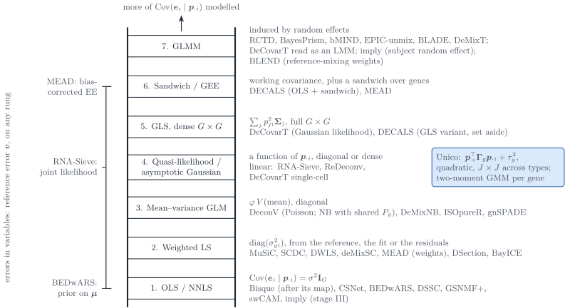
Figure 4: The ladder of noise models for the bulk error \boldsymbol{e}_i of Eq. 6, from the least structured covariance (rung 1, bottom) to the most structured (rung 7, top). Beside each rung, the working \operatorname{Cov}(\boldsymbol{e}_i\mid\boldsymbol{p}_{\cdot i}) and the reviewed methods. Unico (highlighted) sits on rung 4 with a variance quadratic in \boldsymbol{p}_{\cdot i}, through a J\times J covariance across cell types, fitted by a two-moment generalised method of moments. DeconV sits on rung 3; imply (subject random effect) and BLEND (random reference-mixing weights) on rung 7, imply also on rung 1 for its final proportions. The bracket on the left marks the errors-in-variables layer, which can be added on any rung.

Errors in variables cuts across the ladder: the regressor error \boldsymbol{v} of Eq. 6 can be added on any rung, as a joint likelihood (RNA-Sieve, rung 4), a bias-corrected estimating equation (MEAD, rung 6) or a prior on the signature (BEDwARS, rung 1).

Table 3: A ladder of noise models for the bulk error, from the least to the most structured covariance. A method appears on more than one rung when its point estimate and its interval use different covariance models.

Rung	\operatorname{Cov}(\boldsymbol{e}_i\mid\boldsymbol{p}_{\cdot i})	Reviewed methods	Interval for \boldsymbol{p}_{\cdot i}
1. OLS / NNLS	\sigma^{2}\mathbf{I}_G	Bisque (after its gene-wise map), CSNet (both moment regressions), BEDwARS, DSSC, GSNMF+, swCAM, imply (stage III, with subject references)	none, or posterior (BEDwARS)
2. WLS	diagonal	MuSiC, SCDC, DWLS, deMixSC, MEAD (weights), DSection, BayICE	none when the weights are re-estimated from residuals
3. Mean–variance GLM	\varphi V(\text{mean}), diagonal	DeconV (Poisson, or negative binomial with a shared P_g), DeMixNB (negative binomial), ISOpureR, gnSPADE (multinomial)	Fisher information or posterior
4. QL / asymptotic Gaussian	function of \boldsymbol{p}_{\cdot i} (linear: RNA-Sieve, ReDeconv, DeCovarT single-cell; quadratic: Unico)	RNA-Sieve (composite), ReDeconv, Unico (moments, J\times J across types), DeCovarT single-cell (dense, linear in \boldsymbol{p}_{\cdot i})	Fisher or Godambe; not applicable for Unico, whose \boldsymbol{p}_{\cdot i} is given
5. GLS, dense	full G\times G	DECALS (GLS variant, set aside by its authors), DeCovarT (\sum_jp_{ji}^{2}\boldsymbol{\Sigma}_j, Gaussian likelihood)	Wald from the Fisher information, bootstrap
6. Sandwich / GEE	working, plus sandwich	DECALS (OLS + sandwich), MEAD	sandwich, G\to\infty
7. GLMM	induced by random effects	RCTD, BayesPrism, bMIND, EPIC-unmix, BLADE, DeMixT, imply (subject random effect, stage II), BLEND (random reference-mixing weights); DeCovarT read as a linear mixed model (LMM reading)	likelihood or posterior

Moment estimators give point estimates. Weighted non-negative least squares (MuSiC, SCDC, DWLS, deMixSC) solves the normal equations \hat{\boldsymbol{\mu}}^{\top}\boldsymbol{W}(\boldsymbol{y}_{\cdot i}-\hat{\boldsymbol{\mu}}\boldsymbol{p}_{\cdot i})=\boldsymbol{0}, and Unico matches first and second sample moments explicitly. All are generalised method of moments estimators: consistent under correct moment conditions, but they return a point estimate only. An interval needs a higher rung: a sandwich (DECALS, MEAD), a likelihood (RNA-Sieve, DeCovarT) or a resampling unit (genes, cells or donors). When the weights are re-estimated from the residuals of the same fit (MuSiC, deMixSC), the nominal weighted-least-squares covariance is not valid either (our remark).

Families of multivariate models

Here multivariate means several correlated responses per unit, the G genes of one bulk sample; it is not multivariable, which refers to several explanatory variables. Rungs 5 to 7 need a joint law, or at least a joint covariance, for those G responses. Two families supply one (Agresti 2015, sec. 9.1).

• Marginal models specify \mathbb{E}(\boldsymbol{y}_{\cdot i}\mid\boldsymbol{p}_{\cdot i}) and the dependence between genes directly. An explicit joint law that accepts any positive-definite covariance and stays in its family under marginalisation and conditioning is essentially the Gaussian, with its scale mixtures such as the multivariate t, where a zero in the precision no longer means conditional independence (our summary). For counts, many joint laws share the same margins, none is canonical, and the number of parameters grows quickly: a trivariate Poisson built from sums of independent Poisson variables already needs seven of them (Olkin 1994, pp. 37 and 42–43 ). A marginal model of bulk expression therefore takes one of three routes: an asymptotic Gaussian (RNA-Sieve, ReDeconv, DeCovarT single-cell); moments only, through quasi-likelihood or GEE (DECALS, MEAD); or a copula, which couples chosen univariate margins into a full likelihood (none of the reviewed deconvolution methods).
• Conditional models specify the law given latent effects and let shared effects induce the correlation: the GLMMs of rung 7 (RCTD, BayesPrism) and the Poisson–log-normal family of
  1. The integrated margins leave the conditional family (a Poisson–log-normal count is not Poisson), and a zero in the latent precision is a conditional independence between latent log-expressions, not between counts.

For Gaussian responses with an identity link the two families meet. A linear mixed model \boldsymbol{y}=\mathbf{X}\boldsymbol{\beta}+\mathbf{Z}\boldsymbol{u}+\boldsymbol{\epsilon}, with \boldsymbol{u}\sim\mathcal{N}(\boldsymbol{0},\mathbf{G}_u) and \boldsymbol{\epsilon}\sim\mathcal{N}(\boldsymbol{0},\mathbf{R}), implies the marginal model \mathcal{N}(\mathbf{X}\boldsymbol{\beta},\mathbf{Z}\mathbf{G}_u\mathbf{Z}^{\top}+\mathbf{R}), whose fixed effects GLS estimates (Agresti 2015, sec. 9.2–9.3). DeCovarT sits at that point: its Gaussian convolution is a marginal model and, read conditionally, a linear mixed model whose random-effect design depends on \boldsymbol{p}_{\cdot i} (LMM reading). With a non-identity link the conditional and the population-averaged coefficients differ, so a count-scale DeCovarT would have to choose between the two families.

Univariate methods: genes independent

MuSiC

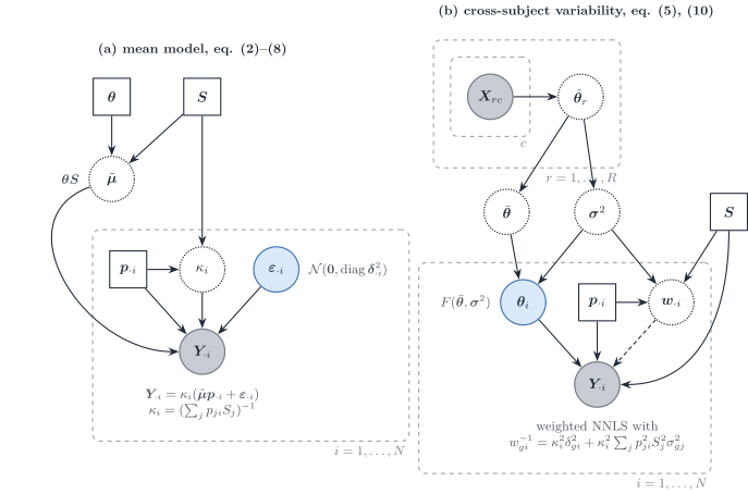
Figure 5: MuSiC (Wang et al. 2019) in this vignette’s notation. (a) The mean model: bulk relative abundance is a cell-size-weighted mixture of relative profiles \boldsymbol{\theta}, rescaled by \kappa_i. (b) The multi-subject reference: subject-level relative profiles \boldsymbol{\theta}_i vary around the cross-subject mean with variance \boldsymbol{\sigma}^{2}, and the inverse of the resulting gene variance weights a non-negative least squares fit.

MuSiC starts from molecules: the bulk of subject i holds X_{gi}=\sum_jm_{ji}S_j\theta_{gj}=\sum_jm_{ji}\tilde\mu_{gj}, with S_j the mean total molecules per cell of type j (equation 2). It works on relative abundance Y_{gi}=X_{gi}/\sum_{g'}X_{g'i}, so that, with the reparametrisation above,

Y_{gi}=\kappa_i\Bigl(\sum_jp_{ji}S_j\theta_{gj}+\varepsilon_{gi}\Bigr), \qquad \operatorname{Var}(Y_{gi}\mid\boldsymbol{p}_{\cdot i}) =\kappa_i^{2}\delta_{gi}^{2}+\kappa_i^{2}\sum_jp_{ji}^{2}S_j^{2}\sigma^{2}_{gj} =w_{gi}^{-1} \tag{7}

(equations 8–10). The second term comes from subject-level relative profiles \theta_{gj,i}\sim F(\theta_{gj},\sigma^{2}_{gj}) (assumption A1): it is the diagonal of the between-replicate layer \boldsymbol{S}_B(\boldsymbol{p}), quadratic in p_{ji}, and it requires a multi-subject reference. Cross terms between types are dropped, which implicitly assumes independence across types. \delta^{2}_{gi} is the residual variance of the bulk. The within-type cell scatter \boldsymbol{\Sigma}_{W,j} has no term in Eq. 7; it is used only to select genes with small within-cluster variance in the tree-guided recursion; the cross-subject weights and the cross-cell selection are the two halves of what the paper calls marker-gene consistency (p. 2). Estimation is weighted non-negative least squares, with the weights updated from an initial fit because \delta^{2}_{gi} is unknown, followed by rescaling to the simplex.

Scales and identifiability. S_j is plugged in as the mean library size of type j in the reference. That substitution returns cell fractions only under assumption A3', a capture efficiency (observed library size over molecule content) common to all types (the MuSiC assumptions); otherwise MuSiC estimates the RNA-weighted product p_{ji}S_j. Under A1–A3 alone the paper claims only the trend of proportions across subjects. Absolute S_j is not needed: it cancels into \kappa_i. A gene- and subject-specific intercept \alpha_{gi} absorbs protocol bias. MuSiC2 keeps the weights and removes genes that are differentially expressed between the reference and bulk conditions (Fan et al. 2022).

Ladder and errors in variables (Sec. 2.3, Sec. 2.2): rung 2; response error only, with a diagonal variance quadratic in \boldsymbol{p}_{\cdot i}; \hat{\boldsymbol{\mu}} is plugged in, and the estimator is a weighted moment estimator.

SCDC

SCDC keeps the weighted non-negative least squares of MuSiC and changes the weights and the reference (Dong et al. 2021). Each gene receives a maximal variance weight, “so that residuals from genes with larger weights have smaller impact” (p. 5): as we read the formula (garbled in our copy, p. 9), the largest cross-cell variance of the gene over the cell types of one reference subject, divided by its median over genes. Weights below the 15th percentile are raised to it and weights above the 85th percentile are lowered to it (p. 10), so the clipping is a percentile rule, not an influence diagnostic. With several single-cell references, SCDC fits each one separately and combines the estimates with data-set weights chosen to fit the bulk (its ENSEMBLE step). No interval for \boldsymbol{p}_{\cdot i} is reported.

Ladder and errors in variables (Sec. 2.3, Sec. 2.2): rung 2; response error only; a weighted moment estimator with no interval.

RNA-Sieve

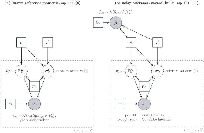
Figure 6: RNA-Sieve (Erdmann-Pham et al. 2021). (a) With known per-cell moments (\tilde{\boldsymbol{\mu}},\boldsymbol{\varsigma}^{2}), the bulk is the sum of n_i cells drawn from the cell mixture, with a central-limit Gaussian per gene whose variance is the mixture variance. (b) The reference means are themselves noisy averages of C_j cells; the joint likelihood over bulks and reference means is maximised, with Godambe sandwich intervals.

RNA-Sieve writes the bulk as a sum of n cells, each a draw from the cell mixture the mixture-of-cells covariance restricted to one gene. By the central limit theorem,

y_{gi}\sim\mathcal{N}\bigl(n_i(\tilde{\boldsymbol{\mu}}\boldsymbol{p}_{\cdot i})_g,\ n_i\sigma^{2}_{gi}\bigr), \qquad \sigma^{2}_{gi}=\sum_jp_{ji}\bigl(\varsigma^{2}_{gj}+\tilde\mu_{gj}^{2}\bigr)-(\tilde{\boldsymbol{\mu}}\boldsymbol{p}_{\cdot i})_g^{2}, \tag{8}

with genes independent (equations 5–8). The variance is linear in n_i and in \boldsymbol{p}, minus the square of the mixture mean: the within-type variance \sum_jp_{ji}\varsigma^{2}_{gj} plus the spread of the type means, the diagonal of the mixture-of-cells covariance. The reference means are noisy, \hat{\tilde\mu}_{gj}\sim\mathcal{N}(\tilde\mu_{gj},\varsigma^{2}_{gj}/C_j) (equation 9), and the true means are estimated jointly with (\boldsymbol{p}_{\cdot i},n_i) from all bulks (equations 10–11). Marginalising them instead would add n_i^{2}\sum_jp_{ji}^{2}\varsigma^{2}_{gj}/C_j to the variance, a quadratic term that vanishes as the reference grows (our remark).

Here \varsigma^{2}_{gj} is the per-cell variance of gene g in type j, the diagonal of \boldsymbol{\Sigma}_{W,j}.

Scales. Raw counts keep S_j inside \tilde{\boldsymbol{\mu}}, so the weights are cell fractions; the optional rescaling of every cell to the median library size removes S_j and turns them into RNA fractions. Any global protocol difference is absorbed into n_i, which then “loses interpretability” as a cell number across protocols (Supplementary S1.4). The optional cell QC drops cells whose library size lies 3 median absolute deviations or more from the median of their type; the gene filters are compared in the feature-selection review.

Intervals. When the model holds, the inverse Fisher information of (\hat{\boldsymbol{p}}_{\cdot i},\hat n_i), after a reparametrisation of the simplex, gives \chi^{2}_{J-1} ellipsoids. Under protocol shift the data law leaves the model family, and the default Godambe sandwich describes the fluctuations around the Kullback–Leibler projection onto that family; without misspecification the two matrices coincide (Godambe 1960). Near-collinear cell types make the information nearly singular. The paper notes that gene correlation “may be incorporated” once it is known, but does not implement it: the product over genes is a composite likelihood.

Against DeCovarT. DeCovarT draws one latent profile per type and keeps a full gene–gene covariance, \sum_jp_{ji}^{2}\boldsymbol{\Sigma}_j, where RNA-Sieve sums n_i cells gene by gene. DeCovarT already has the Fisher analogue, the expected information mapped through the ILR chart (interior intervals), undefined on a face of the simplex. A Godambe correction matters only if the Gaussian convolution is misspecified (counts, protocol shift, omitted types); its one-column construction is a proposal, not implemented (sandwich for a misspecified convolution). It replaces neither the boundary tests nor reference_bootstrap_decovart(), the resampling counterpart of the noisy-reference term.

Ladder and errors in variables (Sec. 2.3, Sec. 2.2): rung 4, a composite asymptotic Gaussian; both layers, the response error with a central-limit law over cells and the regressor error in a joint likelihood.

DWLS

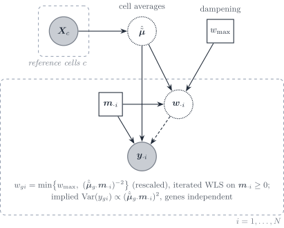
Figure 7: DWLS (Tsoucas et al. 2019). The signature is the average of reference cells; the bulk is fitted in cell-type numbers \boldsymbol{m}_{\cdot i} by iterated weighted least squares, with weights equal to the inverse squared fitted mean, capped by a dampening constant w_{\max}.

DWLS fits the cell-type numbers \mathbf{x}=\boldsymbol{m}_{\cdot i} by

\hat{\boldsymbol{m}}_{\cdot i} =\arg\min_{\boldsymbol{m}\ge\boldsymbol{0}}\sum_g\bar w_{gi}\bigl(y_{gi}-\hat{\tilde{\boldsymbol{\mu}}}_{g\cdot}\boldsymbol{m}\bigr)^{2}, \qquad \bar w_{gi}=\min\Bigl\{w_{\max},\ \frac{(\hat{\tilde{\boldsymbol{\mu}}}_{g\cdot}\hat{\boldsymbol{m}}_{\cdot i})^{-2}}{\min_{g'}(\hat{\tilde{\boldsymbol{\mu}}}_{g'\cdot}\hat{\boldsymbol{m}}_{\cdot i})^{-2}}\Bigr\}, \tag{9}

iterated from an ordinary least squares start, with w_{\max}=2^{q} chosen to minimise the variance of estimates over random half-gene subsets (equations 6–15). The purpose is stated on p. 7: with weights 1/(\text{fitted expression})^{2} the loss becomes a function of the relative error of each cell type, “because we would like all cell types to be estimated with equal accuracy”; highly expressed genes, which dominate an unweighted fit and favour abundant types, are down-weighted. Read as a variance model, the weights imply \operatorname{Var}(y_{gi})\propto(\hat{\tilde{\boldsymbol{\mu}}}_{g\cdot}\boldsymbol{m}_{\cdot i})^{2}, a constant coefficient of variation, which the paper does not state. There is no \boldsymbol{\Sigma}_{W,j} term and genes are independent. \mathbf{x} are cell numbers only under equal RNA per cell; otherwise they are RNA-weighted.

Ladder and errors in variables (Sec. 2.3, Sec. 2.2): rung 2, with a variance proportional to the squared mean (the variance function of a gamma GLM, our reading); response error only; a weighted moment estimator with no interval.

deMixSC

deMixSC keeps the weighted non-negative least squares of MuSiC and DWLS and adds a small benchmark data set: bulk and single-nucleus libraries prepared from the same nucleus aliquot, so that the real bulk and the pseudo-bulk share the composition (Guo et al. 2025, p. 149 ; preprint Guo et al. (2023)). In the 24 benchmark retinas, more than 5000 genes differ between the two platforms in each batch, and TPM normalisation does not remove the difference. In our notation the working model is (supplementary note, equations S.1–S.5, pp. 1–2)

y_{gi}=n_i\sum_jp_{ji}\tilde\mu_{gj}+\epsilon_{gi}, \qquad \tilde\mu_{gj}=S_j\theta_{gj}, \qquad \hat{\tilde\mu}_{gj}=\tilde\mu_{gj}+\bar\xi_{gj}, \tag{10}

with mean-zero bulk noise \epsilon_{gi} and an averaged single-cell measurement error \bar\xi_{gj}. The residual of a fit with \hat{\tilde{\boldsymbol{\mu}}} is the estimation error plus a “technological discrepancy” between platforms (note, p. 3). Two changes to weighted NNLS follow.

• Partitioned loss (equation S.7, note p. 3). Genes differentially expressed between real bulk and pseudo-bulk in the benchmark (paired t-test, Benjamini–Hochberg adjusted P<0.05, the 5000 most expressed of them by default) form a set G_2. They are kept, not removed: their bulk value and reference are divided by a constant a (1000 by default), which scales their squared residuals by a^{-2}:

  \hat{\boldsymbol{p}}_{\cdot i}=\arg\min_{\boldsymbol{p}\ge\boldsymbol{0}} \sum_{g\in G_1}w_{gi}\,r_{gi}(\boldsymbol{p})^{2} +\frac{1}{a^{2}}\sum_{g\in G_2}w_{gi}\,r_{gi}(\boldsymbol{p})^{2}, \qquad r_{gi}(\boldsymbol{p})=y_{gi}-n_i\sum_jp_{ji}\hat{\tilde\mu}_{gj}. \tag{11}

• Weights (equation S.9, note p. 3; main text p. 150): w_{gi}^{-1}=\hat y_{gi}^{2}+(y_{gi}-\hat y_{gi})^{2}+c, with \hat y_{gi}=n_i\sum_j\hat p_{ji}\hat{\tilde\mu}_{gj} and c=2. Earlier methods, the authors note, use “either the squared fitted value” (DWLS, Eq. 9) “or the variance” (MuSiC’s iteratively estimated \delta^{2}_{gi}, Eq. 7), “but never both” (p. 157). The fit is iterated from an NNLS start (note, p. 4).

The target cohort is first aligned to the benchmark bulk by quantile normalisation and ComBat (p. 150). The platform effect is treated as noise to down-weight, not as a gene-wise ratio \tilde b_g to estimate: with a=1000 the genes of G_2 receive a weight 10^{-6} times smaller, which nearly discards them. The squared residual in the weight uses one residual per gene as its own variance, an outlier-damping device in the spirit of robust M-estimation rather than a variance model (our reading). Cell size enters through \tilde\mu_{gj}=S_j\theta_{gj}, as in MuSiC, so \hat{\boldsymbol{p}} are cell fractions under the same equal-efficiency assumption. No interval is reported.

Ladder and errors in variables (Sec. 2.3, Sec. 2.2): rung 2; both layers are written down but enter only through the weights; a weighted moment estimator with no interval.

Bisque

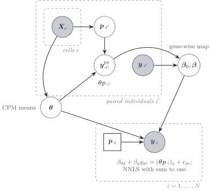
Figure 8: Bisque (Jew et al. 2020), paired mode. For individuals with both assays, the single-cell counts give a CPM signature \boldsymbol{\theta} and counted proportions, hence a pseudo-bulk; a gene-wise linear map from observed bulk to pseudo-bulk is learned on those pairs and applied to the remaining bulks before non-negative least squares.

Bisque learns the platform shift instead of modelling it. In paired mode it fits y^{\mathrm{ps}}_{gi'}=\beta_{0g}+\beta_gy_{gi'}+\epsilon_{gi'} per gene, with \boldsymbol{y}^{\mathrm{ps}}_{\cdot i'}=\boldsymbol{\theta}\boldsymbol{p}_{\cdot i'} the pseudo-bulk of individual i' (equation 1); in unpaired mode it matches the first two moments of each gene across samples (equations 2–3). The transformed bulk is then fitted by non-negative least squares with a sum-to-one constraint. The fitting step has homoscedastic residuals; the variability of the reference enters only through the between-sample moments used in the map. Because \boldsymbol{\theta} is built from CPM, cell size is removed from the signature; the gene-wise affine map absorbs the platform ratio \tilde b_g (as 1/\beta_g) and an intercept, not a type-specific S_j. In unpaired mode the cohort mean composition is assumed equal to the mean composition of the single-cell individuals.

Ladder and errors in variables (Sec. 2.3, Sec. 2.2): rung 1; the platform error is removed by a learned map, then a homoscedastic moment estimator; no interval.

Perspective: two-scale transport beyond the gene-wise map

Perspective

Not implemented. DeCovarT learns its sample scales inside the likelihood (2.1, alignment; 2.1, profile Newton). This subsection says what a richer alignment would add.

Bisque states its goal per gene: “For each gene j, our goal is to transform the observed bulk expression across all n bulk samples X_j\in\mathbb{R}^n to match the mean and variance of Y_j\in\mathbb{R}^{n'}; hence, the transformation of X_j will be a linear transformation” (Jew et al. 2020, 10). Here Y_j is the pseudo-bulk of the n' single-cell individuals. Without pairs, the map is X_{j,\mathrm{transformed}}=(X_j-\bar X_j)\,\hat\sigma_j/\sigma_{X_j}+\bar Y_j, with \hat\sigma_j^{2} a shrunk variance of Y_j (equations 2–3, p. 10). The authors name the price: “a key assumption of our transformation framework is that single-cell-based estimates of cell proportions accurately reflect the true proportions we wish to estimate” (p. 9).

Our reading, not the authors’: equation 3 is, gene by gene, the optimal transport map between two univariate Gaussians. Between \mathcal{N}(\boldsymbol{m}_1,\boldsymbol{\Sigma}_1) and \mathcal{N}(\boldsymbol{m}_2,\boldsymbol{\Sigma}_2) the quadratic-cost map is affine,

T(\boldsymbol{x})=\boldsymbol{m}_2+\boldsymbol{A}(\boldsymbol{x}-\boldsymbol{m}_1), \qquad \boldsymbol{A}=\boldsymbol{\Sigma}_1^{-1/2}\bigl(\boldsymbol{\Sigma}_1^{1/2}\boldsymbol{\Sigma}_2\boldsymbol{\Sigma}_1^{1/2}\bigr)^{1/2}\boldsymbol{\Sigma}_1^{-1/2}, \tag{12}

with cost W_2^2=\lVert\boldsymbol{m}_1-\boldsymbol{m}_2\rVert^2+\operatorname{tr}\{\boldsymbol{\Sigma}_1+\boldsymbol{\Sigma}_2-2(\boldsymbol{\Sigma}_1^{1/2}\boldsymbol{\Sigma}_2\boldsymbol{\Sigma}_1^{1/2})^{1/2}\} (Knott and Smith 1984; Dowson and Landau 1982). For diagonal covariances \boldsymbol{A} is diagonal with entries \sigma_{2g}/\sigma_{1g}, which is Bisque’s map. Bisque is thus Gaussian transport with genes independent, applied to the law of the mixed bulk across samples. That law depends on the composition of each cohort, hence the assumption quoted above.

Transport of type-level laws avoids the composition. With the hierarchy of 2.1, three regimes there are two laws per type, and so two scales (Figure 9):

• cell scale: cells of type j in specimen r, \mathcal{N}(\boldsymbol{M}_{jr},\boldsymbol{\Sigma}_{W,j}). A map S_j aligns them across single-cell platforms, for example nuclei against whole cells;
• type scale: type-level profiles across specimens, \mathcal{N}(\tilde{\boldsymbol{\mu}}_{\cdot j},\boldsymbol{\Sigma}_{B,j}). A map T_j carries this law to the bulk platform, against an external population Gaussian such as sorted profiles or a many-donor pseudo-bulk atlas.

The mean of C cells has covariance \boldsymbol{\Sigma}_{B,j}+\boldsymbol{\Sigma}_{W,j}/C, so S_j and T_j differ even when the two covariances share structure; one transport does not serve both. The three maps form a ladder:

Table 4: Restrictions of an affine platform map, from the one DeCovarT fits to full Gaussian transport.

Map of a type-level law	Free parameters	Where
Scalar, \boldsymbol{x}\mapsto a\boldsymbol{x}	1 per bulk sample	DeCovarT, inside the likelihood (2.1)
Diagonal, gene-wise affine	2G	Bisque, on the mixed bulk; platform ratio \tilde{\boldsymbol{b}} of 2.1
Full affine, Eq. 12	G+G(G+1)/2	This perspective

Any map richer than a scalar absorbs \boldsymbol{p}_{\cdot i} if it is fitted on the bulk sample being deconvolved (2.1, alignment). It needs paired samples, an external cohort or an external population law. With one reference specimen \boldsymbol{\Sigma}_{B,j} is not identified (2.1, one replicate), so T_j needs that external law. DecOT uses transport differently, as a loss between count histograms for the composition (Liu et al. 2022).

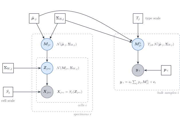
Figure 9: Two-scale transport for one cell type j (perspective). Each specimen r draws a type-level profile \boldsymbol{M}_{jr} from \mathcal{N}(\tilde{\boldsymbol{\mu}}_{\cdot j},\boldsymbol{\Sigma}_{B,j}) (type scale); its cells scatter around it with \boldsymbol{\Sigma}_{W,j} (cell scale). The map S_j carries latent cells to the reference platform. The map T_j pushes the type-level law to the bulk platform, where bulk sample i mixes the transported profiles; \boldsymbol{\epsilon}_i collects within-type cell noise and bulk measurement noise. Bisque instead applies a diagonal map to the mixed bulk.

RCTD

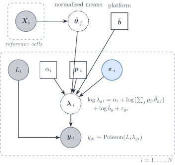
Figure 10: RCTD (Cable et al. 2022) in this vignette’s notation. The reference is collapsed to fixed normalised means \hat{\boldsymbol{\theta}}_{\cdot j}. Sample i carries an observed depth L_i, a leftover scale \alpha_i, a composition and a gene-wise overdispersion; the platform ratio \tilde{\boldsymbol{b}} is shared across samples and is not estimated inside the per-sample fit.

RCTD works one layer below DeCovarT. Each UMI first picks a type with probability p_{ji}, then a gene from that type’s relative profile: a read-level mixture, not a convolution of random population profiles (Cable et al. 2022). Given the rate, gene counts are Poisson; the rate is log-normal around a linear mixture of the fixed normalised means \theta_{gj} (supplementary equations 3, 22):

y_{gi}\mid\lambda_{gi}\sim\mathrm{Poisson}(L_i\lambda_{gi}), \qquad \log\lambda_{gi}=\alpha_i+\log\Bigl(\sum_jp_{ji}\theta_{gj}\Bigr)+\gamma_g+\varepsilon_{gi}, \tag{13}

with L_i the observed depth, \alpha_i a leftover sample scale, \gamma_g\sim\mathcal{N}(0,\sigma_\gamma^{2}) a gene-specific platform random effect and \varepsilon_{gi}\sim\mathcal{N}(0,\sigma_\varepsilon^{2}) an observation-level random effect, with heavier tails in practice (p. 6). The model is a Poisson–log-normal GLMM. The Poisson mean is

\mathbb{E}[y_{gi}\mid\varepsilon_{gi}] =\underbrace{L_ie^{\alpha_i}}_{a_i}\,\tilde b_g\,e^{\varepsilon_{gi}}\sum_jp_{ji}\theta_{gj}, \qquad \tilde b_g=e^{\gamma_g}, \tag{14}

so the platform effect is exactly the gene-wise ratio \tilde b_g of Sec. 1.1, and \varepsilon_{gi} is the count-scale analogue of a diagonal bulk residual. Genes are independent given \varepsilon. In the language of the measurement model, the rate of gene g is a type-weighted sum of per-type rates scaled by one sample-wide factor; the same holds in DeCovarT’s single-cell mean a_in_i\tilde{\boldsymbol{\mu}}\boldsymbol{p}_{\cdot i}, whose per-type contribution is n_ip_{ji}S_j molecules of profile \boldsymbol{\theta}_{\cdot j} (our reading). A mixture is the right story at the UMI; a convolution of random profiles (Eq. 20) is the right story for population profiles.

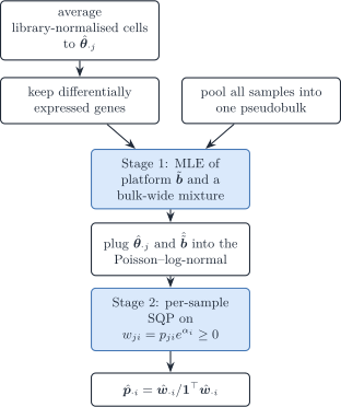
Figure 11: RCTD estimation. Stage 1 identifies the gene-wise platform ratio from a pseudobulk of all samples; stage 2 fits each sample by sequential quadratic programming on the unnormalised weights w_{ji}=p_{ji}e^{\alpha_i}.

The fit is two-stage because \tilde{\boldsymbol{b}} cannot be free inside one sample (alignment scales): stage 1 estimates \sigma_\gamma and predicts \gamma_g from one pseudobulk of all spots (supplementary equations 14–19), stage 2 holds it fixed. That is Strategy 4 in its purest form (plug-in scales). Stage 2 maximises a non-convex Poisson–log-normal likelihood in w_{ji}=p_{ji}e^{\alpha_i}\ge0 by sequential quadratic programming: the Hessian is replaced by its positive-semidefinite part and each step is a constrained quadratic programme with step size 0.3. Zeros on the orthant boundary are native to that formulation, which suits spots with few types. DeCovarT instead maps \boldsymbol{p} to the ILR chart and takes Newton–Raphson steps with the analytic score and Hessian of a Gaussian law.

Ladder and errors in variables (Sec. 2.3, Sec. 2.2): rung 7, a Poisson–log-normal GLMM; response error only; the reference means are plugged in and the platform effect is predicted in stage 1, then held fixed.

DeconV

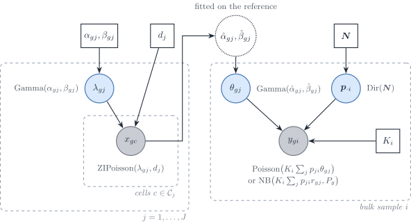
Figure 12: DeconV (Gynter et al. 2023) in this vignette’s notation, Poisson (“gamma”) variant. Left, the reference model, fitted first: the counts of cell c of type j are zero-inflated Poisson with a Gamma-distributed rate and a type-specific dropout d_j. Right, the bulk model: the fitted hyperparameters give a Gamma rate \theta_{gj} per type, the proportions follow a Dirichlet whose concentration \boldsymbol{N} is fitted, and the bulk count is Poisson with a mean linear in \boldsymbol{p}_{\cdot i}. The negative-binomial variant replaces \theta_{gj} by a log-normal r_{gj} and adds a gene-wise P_g shared by all types.

DeconV fits a count model to the single-cell reference, then aggregates it to the bulk (Gynter et al. 2023). The reference model (equations 1–2, p. 6) takes the counts of a cell c of type j as zero-inflated Poisson, x_{gc}\sim\mathrm{ZIPoisson}(\lambda_{gj},d_j), or zero-inflated negative binomial, \mathrm{ZINB}(r_{gj},P_g,d_j), with priors \lambda_{gj}\sim\mathrm{Gamma}(\alpha_{gj},\beta_{gj}), r_{gj}\sim\mathrm{LogNormal}(\mu_{gj},\sigma_{gj}) and P_g\sim\mathrm{Beta}(\alpha_g,\beta_g). The hyperparameters and the dropout are fitted by maximum likelihood on mini-batches of cells. The bulk model (equations 3–5, pp. 6–7) is

\theta_{gj}\sim\mathrm{Gamma}(\hat\alpha_{gj},\hat\beta_{gj}), \qquad y_{gi}\sim\mathrm{Poisson}\Bigl(K_i\sum_jp_{ji}\theta_{gj}\Bigr), \qquad \boldsymbol{p}_{\cdot i}\sim\mathrm{Dirichlet}(\boldsymbol{N}), \tag{15}

or y_{gi}\sim\mathrm{NB}\bigl(K_i\sum_jp_{ji}r_{gj},P_g\bigr) with r_{gj} and P_g drawn from their fitted priors. K_i is “proportional to the number of cells sequenced and the sequencing depth of the bulk sample” (p. 6). Five dropout configurations, with or without zero inflation of the bulk, are offered (Table S1, p. 14); the bulk dropout, when kept, is d_g=\sum_jp_{ji}d_{gj} (equation 6, p. 7). Only the Dirichlet concentration \boldsymbol{N} is fitted on the bulk; the reference hyperparameters stay fixed (p. 7). Both stages run in Pyro with Adam, clipped gradients and learning-rate decay (pp. 7–8). The 95% intervals of Fig. 3 (p. 11) are read from \mathrm{Dir}(\hat{\boldsymbol{N}}), “the distribution for bulk cell type proportions” (p. 7). The paper describes that fit as gradient steps on the log-likelihood under draws from the Dirichlet and states no variational objective, so the calibration of these intervals cannot be judged from the text (our remark). Genes are independent, and no covariance is modelled.

Aggregation, and when it is exact. The Poisson bulk rests on “the sum of two (or more) Poisson random variables has also a Poisson distribution” (p. 6). If a bulk holds m_{ji} cells of type j whose counts of gene g are independent \mathrm{Poisson}(\theta_{gj}), the total is \mathrm{Poisson}(\sum_jm_{ji}\theta_{gj}), which is Eq. 15 with K_i\propto n_i: an exact convolution of univariate Poissons. The negative-binomial bulk is exact only because P_g is shared by all types: a sum of independent \mathrm{NB}(r_c,P) variables is \mathrm{NB}(\sum_cr_c,P), so m_{ji} cells of type j add up to \mathrm{NB}(\sum_jm_{ji}r_{gj},P_g). With a type-specific P_{gj} the sum is no longer negative binomial, and its law is a finite convolution of the kind DeMixNB evaluates (Sec. 5) (our remark). In the Poisson variant, \theta_{gj} is drawn once per bulk, so every cell of a type shares one rate: the Gamma layer is a random population profile, and \operatorname{Var}(y_{gi})=K_i\sum_jp_{ji}\mathbb{E}\theta_{gj}+K_i^{2}\sum_jp_{ji}^{2}\operatorname{Var}\theta_{gj} adds a term quadratic in p_{ji} to the Poisson term, gene by gene (our reading).

Relation to deMixSC, DeMixNB and DeCovarT. deMixSC writes the bulk the same way, as a sum over the cells of each type (supplementary note, equations S.1–S.2, pp. 1–2; Eq. 10), but adds a mean-zero bulk noise with no law and fits weighted NNLS: it uses the sum for the mean only, and it is not a negative-binomial convolution. DeMixNB is the exact convolution of two negative binomials with their own dispersions (Montierth et al. 2025). DeCovarT convolves Gaussian population profiles and keeps their gene–gene covariance. In that order the variance model grows from a weight (deMixSC, rung 2) to a count law per gene (DeconV, DeMixNB, rung 3) to a dense covariance (DeCovarT, rung 5).

Ladder and errors in variables (Sec. 2.3, Sec. 2.2): rung 3, a Poisson or negative-binomial GLM per gene, with a random Gamma rate or log-normal size; response error only, the reference law is plugged in through its fitted hyperparameters; interval from the fitted Dirichlet.

ReDeconv

ReDeconv names three ways a single-cell reference distorts deconvolution: rescaling every cell to a common total (CP10K), which erases transcriptome size; the gene-length mismatch between UMI single-cell counts and full-length bulk libraries; and ignoring the within-type variance (Lu et al. 2025).

Model. The bulk is a sum of m_{ji} independent cells of each type. By the central limit theorem, after a rescaling of the bulk by a constant c and with weights f_{ji}=cm_{ji},

y_{gi}\sim\mathcal{N}\Bigl(\sum_jf_{ji}\tilde\mu_{gj},\ c\sum_jf_{ji}\sigma^{2}_{gj}\Bigr), \tag{16}

with genes independent, and the composition is estimated by maximising the product of these densities over genes. The variance is linear in the weights, the diagonal of the within-type layer n_i^{-1}\sum_jp_{ji}\boldsymbol{\Sigma}_{W,j} (one replicate), as in RNA-Sieve without the spread of type means. The optimiser, the estimation of c and the final simplex step are not stated.

Transcriptome size. CLTS normalisation fits, for each single-cell sample r, a line S_{jr}=\alpha_rS_{j1}+\beta_r between its mean transcriptome sizes per type and those of a baseline sample, then rescales every count of sample r as x_{gc}\leftarrow x_{gc}/\alpha_r+(v_{\max}-\beta_r/\alpha_r)/G with v_{\max}=\max_r\beta_r/\alpha_r. Differences of transcriptome size between types within a sample are kept; differences between samples are removed. CLTS therefore keeps S_j in \tilde{\boldsymbol{\mu}}_{\cdot j}=S_j\boldsymbol{\theta}_{\cdot j}, so the fitted weights are cell fractions rather than transcript fractions.

Caveats. About 100 signature genes per type are chosen by a t-test against every other type (P<0.05, no multiplicity correction), a fold change of at least 2 and the smallest coefficient of variation (feature-selection review); the synthetic benchmarks draw bulk and reference from the same single-cell source, as the authors acknowledge.

Ladder and errors in variables (Sec. 2.3, Sec. 2.2): rung 4; response error only, with a central-limit law over cells; the reference is plugged in.

Multivariate methods: gene–gene covariance

DECALS

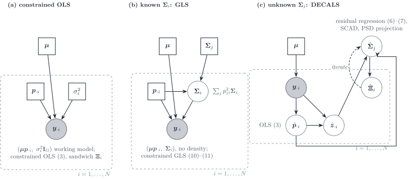
Figure 13: DECALS (Cai et al. 2024) as three increasingly informed working models. (a) Constrained ordinary least squares with an implicit identity covariance; the subject-specific covariance enters only the sandwich variance. (b) Constrained generalised least squares when \boldsymbol{\Sigma}_i=\sum_jp_{ji}^{2}\boldsymbol{\Sigma}_j is known. (c) DECALS proper: the type covariances are unknown and are estimated from bulk residuals across samples, with a bias correction iterated with the variance of \hat{\boldsymbol{p}}_{\cdot i}; the point estimate stays the OLS one.

DECALS makes no distributional assumption on the bulk. Its model (equations 1–2, 5) is

\boldsymbol{y}_{\cdot i}=\sum_jp_{ji}\boldsymbol{x}^{(j)}_i =\boldsymbol{\mu}\boldsymbol{p}_{\cdot i}+\boldsymbol{\epsilon}_i, \qquad \operatorname{Cov}(\boldsymbol{\epsilon}_i)=\boldsymbol{\Sigma}_i=\sum_jp_{ji}^{2}\boldsymbol{\Sigma}_j, \tag{17}

with subject-level type profiles \boldsymbol{x}^{(j)}_i independent across types: exactly the quadratic layer \boldsymbol{S}_B(\boldsymbol{p}) and released DeCovarT’s covariance, without a density. The three panels of Figure 13 are the paper’s three estimators.

1. Constrained OLS (equation 3) is the point estimator. For a large number of genes the inequality constraints are inactive and the estimator is the equality-constrained projection \hat{\boldsymbol{p}}=\mathbf{U}\tilde{\boldsymbol{p}} of the OLS solution (Lemma S1). Its asymptotic covariance is the sandwich \boldsymbol{\Xi}_i=\mathbf{U}\mathbf{D}\mathbf{U}^{\top} with \mathbf{D}=(\tfrac1G\boldsymbol{\mu}^{\top}\boldsymbol{\mu})^{-1}\tfrac1G\boldsymbol{\mu}^{\top}\boldsymbol{\Sigma}_i\boldsymbol{\mu}(\tfrac1G\boldsymbol{\mu}^{\top}\boldsymbol{\mu})^{-1}.
2. Constrained GLS with known \boldsymbol{\Sigma}_i (equations 10–11) is more efficient. The authors reject it once \boldsymbol{\Sigma}_i is estimated: the per-sample inverse square root is too noisy, and the coverage of GLS with an estimated covariance falls to about 0.65–0.8 in their simulations.
3. Unknown \boldsymbol{\Sigma}_j. Because \mathbb{E}[z_{gi}z_{hi}]=\sum_jp_{ji}^{2}\Sigma_{j,gh}, the residual outer products are regressed on the squared proportions across the N samples, \hat{\boldsymbol{c}}_{gh}=(\hat{\mathbf{H}}^{\top}\hat{\mathbf{H}})^{-1}\hat{\mathbf{H}}^{\top}(\hat{\boldsymbol{z}}_g\circ\hat{\boldsymbol{z}}_h) with \hat{\mathbf{H}}=[\hat p_{ji}^{2}] (equation 6), a regression first proposed for known proportions by CSNet. Replacing \mathbf{H} by \hat{\mathbf{H}} deflates the estimate; Proposition 1 gives the bias terms \mathbf{B}_1,\mathbf{B}_2 under a Gaussian approximation of \hat{\boldsymbol{p}}, and the corrected estimator (equation 7) is iterated with \boldsymbol{\Xi}_i, then thresholded by SCAD and projected onto the positive semidefinite cone.

Asymptotics. Genes are the statistical units: Theorem 1 gives \sqrt{G}(\hat{\boldsymbol{p}}_{\cdot i}-\boldsymbol{p}_{\cdot i})\to\mathcal{N}(\boldsymbol{0},\boldsymbol{\Xi}_i) as G\to\infty for one sample, under sub-exponential errors, a dependency graph of bounded degree among genes, and p_{ji}>0 for all types. On a face of the simplex the limit law is not derived. With dense gene correlation the authors report that coverage collapses to about 0.65: the central limit theorem over genes fails when dependence is not sparse. The paper gives no consistency theorem for \hat{\boldsymbol{\Sigma}}_j.

Ladder and errors in variables (Sec. 2.3, Sec. 2.2): rung 6 for the estimate and its interval, with rung 5 as the efficient variant set aside; response error only, with the composition-dependent covariance of DeCovarT; an asymptotic law over genes yields the sandwich interval.

MEAD

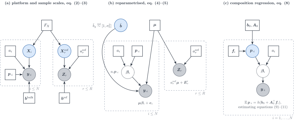
Figure 14: MEAD (Xie et al. 2026) in this vignette’s notation (a_i=\gamma_i, \boldsymbol{b}^{\mathrm{bulk}}=\boldsymbol{\alpha}, \boldsymbol{b}^{\mathrm{ref}}=\boldsymbol{\alpha}^{r}, \boldsymbol{\mu}=\mathbf{U}, replicate r = reference individual j of the paper). (a) Bulk and reference share the population law F_X of the type profiles but have their own sample scales and gene-wise capture factors. (b) After reparametrisation only the ratio \tilde b_g=\alpha_g/\alpha^{r}_g remains, treated as random noise around one, and the bulk mean is \boldsymbol{\mu}\boldsymbol{\beta}_i with \boldsymbol{\beta}_i=a_i\boldsymbol{p}_{\cdot i}. (c) Across individuals, the composition is regressed on covariates.

MEAD is the multivariate errors-in-variables method. Its successive models (Figure 14), translated into our indices, are:

• Scales (equations 2–3). The bulk is \boldsymbol{y}_{\cdot i}=a_i\operatorname{diag}(\boldsymbol{b}^{\mathrm{bulk}})\mathbf{X}_i\boldsymbol{p}_{\cdot i}+\boldsymbol{\epsilon}_i and reference individual r is \mathbf{Z}_r=a^{\mathrm{ref}}_r\operatorname{diag}(\boldsymbol{b}^{\mathrm{ref}})\mathbf{X}^{\mathrm{ref}}_r+\mathbf{E}_r, with \mathbf{X}_i and \mathbf{X}^{\mathrm{ref}}_r drawn from one population law (assumption 1). a_i captures depth and tissue amount, \boldsymbol{b} gene length and GC content. The reference scale is one scalar per reference individual, shared by its cell types (Supplementary S2.1); the authors avoid per-cell library-size normalisation to keep cell size in \boldsymbol{\mu}.

• Reparametrisation (equations 4–5). Only the ratio \tilde b_g=b^{\mathrm{bulk}}_g/b^{\mathrm{ref}}_g is identified, and assumption 3 treats it as noise, \tilde b_g\overset{\text{iid}}{\sim}[1,\sigma_0^{2}], independent of \boldsymbol{\mu}. The model becomes \boldsymbol{y}_{\cdot i}=\boldsymbol{\mu}\boldsymbol{\beta}_i+\boldsymbol{e}_i with \boldsymbol{\beta}_i=a_i\boldsymbol{p}_{\cdot i} and \boldsymbol{e}_i=(\tilde{\boldsymbol{B}}-\mathbf{I})\boldsymbol{\mu}\boldsymbol{\beta}_i+\boldsymbol{\epsilon}'_i: the platform ratio is not estimated, inflates the variance and makes \boldsymbol{e}_i dependent across samples.

• One sample. With \hat a^{\mathrm{ref}}_r=\sum_{j,g}z_{rgj}/(JG) (a plug-in from the reference alone), \hat{\boldsymbol{\mu}}_{g\cdot} the average of \boldsymbol{z}_{rg\cdot}/\hat a^{\mathrm{ref}}_r and \hat{\mathbf{K}}_g its covariance across reference individuals, the bias-corrected estimating equation

  \hat{\boldsymbol{\mu}}^{\top}\mathbf{W}\boldsymbol{y}_{\cdot i}-\bigl(\hat{\boldsymbol{\mu}}^{\top}\mathbf{W}\hat{\boldsymbol{\mu}}-\hat{\mathbf{K}}\bigr)\boldsymbol{\beta}_i=\boldsymbol{0}, \qquad \hat{\mathbf{K}}=\sum_gw_g\hat{\mathbf{K}}_g, \tag{18}

  removes the attenuation caused by a noisy regressor (equation 6). Non-negativity is imposed by truncation or constrained optimisation, and \hat{\boldsymbol{p}}_{\cdot i}=\hat{\boldsymbol{\beta}}_i/\|\hat{\boldsymbol{\beta}}_i\|_1.

• Several samples (section 5). The composition is regressed on covariates, \mathbb{E}[\boldsymbol{p}_{\cdot i}]=h(\boldsymbol{b}_0+\mathbf{A}_0^{\top}\boldsymbol{f}_i), with \hat{\boldsymbol{p}}_{\cdot i} plugged into an estimating equation (11).

• Dependence and weights. Gene–gene dependence is global, not type specific: a dependency graph over genes, estimated from the bulk correlation by a multiple test, enters only the sandwich covariance. The weights w_g=1/\tilde s_g^{2}, with s_g^{2}=\mathbf{1}^{\top}\hat{\mathbf{K}}_g\mathbf{1} shrunk across genes, come from the reference only; MuSiC’s residual-based weights “can severely bias” the estimating equation.

Identifiability (Theorem 1). With a composition matrix of rank J, the proportions are identifiable if and only if \boldsymbol{\mu} has full rank and, for every partition of the genes into t\ge2 blocks, the ranks of the blocks of \boldsymbol{\mu} add to more than J. Perfect marker genes violate the condition: rescaling the platform ratios of the type-j markers by 1/\delta_j, the proportions to \tilde p_{ji}=\delta_jp_{ji}/\sum_\ell\delta_\ell p_{\ell i} and the scale to a_i\sum_\ell\delta_\ell p_{\ell i} leaves the bulk mean unchanged, for any \boldsymbol{\delta}. A gene-wise platform ratio can then mimic a type-specific size factor (Supplementary Remark S1), the \boldsymbol{q} versus \boldsymbol{p} ambiguity of alignment scales; assumption 3 restores identification because a ratio that depends on the type of its marker is no longer independent of \boldsymbol{\mu} (our reading).

Asymptotics. With G\to\infty and the number of reference individuals fixed, Theorems 2–3 give \sqrt{G}(\hat{\boldsymbol{p}}_{\cdot i}-\boldsymbol{p}_{\cdot i})\to\mathcal{N}\bigl(\boldsymbol{0},\nabla g\,\boldsymbol{\Upsilon}^{-1}\boldsymbol{\Sigma}_i\boldsymbol{\Upsilon}^{-1}\nabla g^{\top}\bigr), with the Gram limit \boldsymbol{\Upsilon}=\lim G^{-1}\boldsymbol{\mu}^{\top}\mathbf{W}\boldsymbol{\mu}, when every p_{ji}>0 and the dependency graph is “almost sparse”. The regime is fragile when the reference-noise term does not shrink (fixed number of reference individuals), when types are collinear, at the boundary (the softplus device is inconsistent for finite tuning), and for the composition regression unless N=o(G) (Theorem 4, Remark S3). DECALS reports that MEAD underestimates variances.

Ladder and errors in variables (Sec. 2.3, Sec. 2.2): rung 2 weights inside a rung 6 estimating equation; both layers, the regressor error removed by a bias-corrected estimating equation and the platform ratio a multiplicative response error; the law is asymptotic in G.

Where DeCovarT sits

Released DeCovarT plugs in the mean and gene–gene covariance of each type and fits the Gaussian convolution of Eq. 20, one bulk sample at a time: rung 5 of Table 3, with a covariance that depends on \boldsymbol{p}_{\cdot i} and a full Gaussian likelihood. Against the methods above:

• RNA-Sieve and ReDeconv sum independent cells, so a type’s variance enters linearly in p_{ji}, gene by gene; DeCovarT convolves random population profiles, so it enters quadratically and keeps the gene–gene covariance.
• DECALS assumes the same covariance, \sum_jp_{ji}^{2}\boldsymbol{\Sigma}_j, without a density; its point estimate is least squares and its efficiency depends on how well the covariance is estimated across bulks. MEAD keeps a global gene dependence and adds the platform ratio, but models the reference noise that DeCovarT ignores.
• RCTD is a read-level mixture with gene-wise random effects (rung 7), not a type-level covariance.

For a single-cell reference the bulk is a physical sum of cells, and the variance becomes linear in p_{ji}, as in RNA-Sieve: rung 4 with a dense covariance. The strategies that rebuild DeCovarT for that reference, and the three-layer law that combines within- and between-donor covariances, are in the single-cell generative vignette; the model retained for real data is in the MLE vignette.

Cell-type-specific moments when the composition is known

The methods of Sec. 2 estimate the composition from known reference moments. The reverse problem takes the composition \{\boldsymbol{p}_{\cdot i}\} as known, from any of those methods, and estimates what DeCovarT plugs in: type-level means and covariances, or the purified profile of each type in each sample. Write the convolution with explicit latent profiles,

\boldsymbol{x}_{\cdot j,i}\sim(\boldsymbol{\mu}_{\cdot j},\boldsymbol{\Sigma}_j)\ \text{independent across }j, \qquad \boldsymbol{y}_{\cdot i}=\sum_jp_{ji}\,\boldsymbol{x}_{\cdot j,i}, \tag{19}

so that

\mathbb{E}[\boldsymbol{y}_{\cdot i}]=\boldsymbol{\mu}\boldsymbol{p}_{\cdot i}, \qquad \operatorname{Cov}(\boldsymbol{y}_{\cdot i})=\sum_jp_{ji}^{2}\boldsymbol{\Sigma}_j , \tag{20}

which is the released DeCovarT law when the profiles are Gaussian. Four families use these identities.

• Type-level gene networks across a cohort. CSNet regresses the outer products of bulk residuals on the squared proportions to estimate each \boldsymbol{\Sigma}_j, then thresholds the correlation (Sec. 3.1).
• Sample-level profiles with a covariance across cell types. Unico (Sec. 3.2), and the Bayesian bMIND and EPIC-unmix (Sec. 4.1), place a J\times J covariance \boldsymbol{\Gamma}_g across cell types for each gene, independent across genes. Their covariance is the transpose of DeCovarT’s: it couples types within a gene, not genes within a type.
• Sample-level profiles with a gene–gene covariance. With Gaussian profiles and known moments, the posterior mean of each \boldsymbol{x}_{\cdot j,i} is a Wiener filter, which is also the best linear unbiased predictor of the random effects when Eq. 20 is read as a linear mixed model; both are derived in the Wiener-filter vignette.
• Subject-level references from repeated bulks. imply predicts a profile per subject, shared by that subject’s repeated samples, with a gene-wise linear mixed model, then re-estimates the proportions with it (Sec. 3.3).

On the measurement side, these methods need the bulk on a linear scale (FPKM for CSNet). When the bulk is normalised by its own library size, the known weights act as RNA fractions \boldsymbol{q}_{\cdot i}, not as cell fractions (Sec. 1).

Type-level moments given known proportions

CSNet inverts the DeCovarT arrow (Su et al. 2024). DeCovarT takes (\boldsymbol{\mu},\{\boldsymbol{\Sigma}_j\}) as plug-in and returns \boldsymbol{p}_{\cdot i}. CSNet takes \{\boldsymbol{p}_{\cdot i}\}_{i=1}^{N} as known (from CIBERSORT, MuSiC, or DeCovarT itself) and returns type-level means and a sparse correlation network. The generative identities are the same convolution as Eq. 19 and Eq. 20, written across a cohort rather than one sample:

\mathbb{E}[\boldsymbol{y}_{\cdot i}\mid\boldsymbol{p}_{\cdot i}] = \sum_j p_{ji}\,\boldsymbol{\mu}_{\cdot j}, \qquad \operatorname{Cov}(\boldsymbol{y}_{\cdot i}\mid\boldsymbol{p}_{\cdot i}) = \sum_j p_{ji}^{2}\,\boldsymbol{\Sigma}_j. \tag{21}

No Gaussian law is required for the moments. Let P\in\mathbb{R}^{N\times J} have entries P_{ij}=p_{ji} and H\in\mathbb{R}^{N\times J} have entries H_{ij}=p_{ji}^{2}. Gene-wise ordinary least squares on the linear mean recovers

\hat{\boldsymbol{\mu}}_{g\cdot} = (P^{\top}P)^{-1}P^{\top}\boldsymbol{y}_{g\cdot}, \tag{22}

the bulk analogue of a reference average, now identified from compositional contrast across samples rather than from purified cells. Centred residuals z_{gi}=y_{gi}-\sum_j p_{ji}\hat{\mu}_{gj} then satisfy the pairwise identity z_{gi}z_{g'i}=\sum_j p_{ji}^{2}\Sigma_{gg',j}+\varepsilon_{gg'i}. Least squares of the Hadamard products on H estimates each covariance entry,

\hat{\Sigma}_{gg',j} = \bigl[(H^{\top}H)^{-1}H^{\top}(\boldsymbol{z}_{g\cdot}\odot\boldsymbol{z}_{g'\cdot})\bigr]_{j}. \tag{23}

CSNet converts \hat{\boldsymbol{\Sigma}}_j to a correlation \hat{R}_j and applies an element-wise SCAD threshold. That is a marginal co-expression graph, not a Gaussian Markov precision. The Gaussian convolution log-likelihood in \{\boldsymbol{\Sigma}_j\}, which is the natural DeCovarT loss for the same parameters, is neither convex nor biconvex in those matrices; pairwise least squares is how CSNet avoids that optimisation (Su et al. 2024).

A DeCovarT-native sequel would keep Eq. 22–Eq. 23 as the moment step and map \hat{\boldsymbol{\Sigma}}_j to a sparse precision \boldsymbol{\Omega}_j (network inference), run after \boldsymbol{p} has been estimated (Figure 15). A CSNet correlation graph is not a DeCovarT precision.

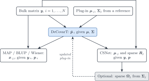
Figure 15: Two inverse problems on the same convolution. DeCovarT estimates p given mu and Sigma. Given p, the MAP / BLUP recovers sample-level purified profiles, and CSNet recovers type-level means and a sparse co-expression network. A precision Omega_j estimated there can be fed back as the DeCovarT plug-in.

P and H must have full column rank, so \boldsymbol{p}_{\cdot i} has to vary across the N bulks. One sample identifies \boldsymbol{p} given (\boldsymbol{\mu},\{\boldsymbol{\Sigma}_j\}); it does not identify J covariance matrices. Rare types with almost constant p_{ji} leave the corresponding column of H weak, which is why CSNet recovers abundant-type co-expression more easily than microglia-scale weights. The method is a moment estimator: modest errors in the supplied \boldsymbol{p} are averaged over N, whereas DeCovarT’s likelihood for a single column is concentrated in \boldsymbol{p}_{\cdot i}.

	DeCovarT	MAP / BLUP (the Wiener filter)	CSNet
Known	\boldsymbol{\mu}_{\cdot j}, \boldsymbol{\Sigma}_j (reference)	\boldsymbol{\mu}_{\cdot j}, \boldsymbol{\Sigma}_j, \boldsymbol{p}_{\cdot i}	\boldsymbol{p}_{\cdot i} (external or DeCovarT)
Unknown	\boldsymbol{p}_{\cdot i}	\boldsymbol{x}_{\cdot j,i} (one sample)	\boldsymbol{\mu}_{\cdot j}, sparse R_j (cohort)
Law	Multivariate Gaussian convolution	Same, posterior of the latents	Moments only; Gaussian optional
Second moment	Sparse precision \boldsymbol{\Omega}_j as input	Uses \boldsymbol{\Sigma}_j, does not re-estimate it	Sparse correlation R_j as output
Replication	One bulk column is enough	One bulk column	N\gg J bulks with varying \boldsymbol{p}
Estimator	Constrained MLE on the ILR chart	Posterior mean / Wiener gain	Gene-wise OLS, then pairwise LS, then SCAD

Ladder and errors in variables (Sec. 2.3, Sec. 2.2): the reverse problem, with the composition known and the latent profiles’ moments as the target; rung 1 regressions for both moments.

Sample-level profiles with a covariance across cell types

Unico (Chen et al. 2025) takes the proportions as given, estimated beforehand by a reference-based method, and estimates for each gene the moments of the latent sample-level profiles, then the profiles themselves (a samples \times genes \times types tensor). Its model (equations 3–6, p. 11), in our notation, makes no distributional assumption:

y_{gi}=\boldsymbol{p}_{\cdot i}^{\top}\boldsymbol{x}_{g\cdot,i}+e_{gi}, \qquad \mathbb{E}\,\boldsymbol{x}_{g\cdot,i}=\boldsymbol{\mu}_{g\cdot}, \quad \operatorname{Cov}\boldsymbol{x}_{g\cdot,i}=\boldsymbol{\Gamma}_g, \qquad \mathbb{E}\,e_{gi}=0, \quad \operatorname{Var}e_{gi}=\tau_g^{2}, \tag{24}

so that \operatorname{Var}(y_{gi})=\boldsymbol{p}_{\cdot i}^{\top}\boldsymbol{\Gamma}_g\boldsymbol{p}_{\cdot i}+\tau_g^{2}.

• Estimator: the model moments of each bulk sample. Each bulk sample has its own law, set by its proportions \boldsymbol{p}_{\cdot i} and the gene parameters \theta_g=\{\boldsymbol{\mu}_{g\cdot},\boldsymbol{\Gamma}_g,\tau_g^{2}\}. Unico therefore does not pool the samples into one empirical moment: each sample contributes one condition per moment, which matches a model moment with that sample’s observation and has mean zero under the model (equations 9–11, p. 13),

  f_{1i}(\theta_g)=\boldsymbol{p}_{\cdot i}^{\top}\boldsymbol{\mu}_{g\cdot}-y_{gi}, \qquad f_{2i}(\theta_g)=\boldsymbol{p}_{\cdot i}^{\top}\boldsymbol{\Gamma}_g\boldsymbol{p}_{\cdot i}+\tau_g^{2}-\bigl(y_{gi}-\boldsymbol{p}_{\cdot i}^{\top}\boldsymbol{\mu}_{g\cdot}\bigr)^{2}. \tag{25}

  The N conditions per moment outnumber the J+J(J+1)/2+1 parameters, so the estimate minimises \boldsymbol{f}^{\top}\hat{\boldsymbol{U}}\boldsymbol{f}, with \hat{\boldsymbol{U}} the inverse covariance of the conditions (equation 12, pp. 13–14) (Hansen 1982). Independent samples make \hat{\boldsymbol{U}} diagonal and the problem weighted least squares; in practice \hat{\boldsymbol{U}} only down-weights samples with large condition values (p. 14).

• Implementation (p. 14). The means are fitted under non-negativity by the constrained least-squares solver pcls of mgcv; the variances and covariances by COBYLA (nloptr), with a small L_2 penalty against the collinearity of the proportions. Samples more than two standard deviations from the gene mean are dropped. The weights are updated after each iteration: two iterations for the means, three for the (co)variances.

• What the moments are taken from. The inputs are the bulk matrix and proportions estimated beforehand (p. 11); Unico needs no single-cell reference. Single cells enter the paper only to build benchmark pseudo-bulks: the type-level pseudo-bulk profiles of one randomly drawn donor are mixed with the proportions of another randomly drawn donor (p. 17), so that the true sample-level profiles are known. Bisque’s unpaired mode (Sec. 2.5.6.1) is different: it matches the mean and variance of each gene across bulk samples with those of single-cell pseudo-bulks, two empirical laws. Unico matches the model moments of each bulk sample with that sample’s observation.

• Profiles. The conditional expectation under a Gaussian working law (Theorem 1, p. 12), \hat{\boldsymbol{x}}_{g\cdot,i}=\boldsymbol{\mu}_{g\cdot}+\boldsymbol{\Gamma}_g\boldsymbol{p}_{\cdot i}(y_{gi}-\boldsymbol{p}_{\cdot i}^{\top}\boldsymbol{\mu}_{g\cdot})/(\boldsymbol{p}_{\cdot i}^{\top}\boldsymbol{\Gamma}_g\boldsymbol{p}_{\cdot i}+\tau_g^{2}), the gene-wise, J\times J analogue of DeCovarT’s Wiener filter; TCA is the case \boldsymbol{\Gamma}_g=\mathbf{I}. Distribution-free asymptotic tests of covariate effects at the cell-type level are offered (Fig. 3b, p. 8).

Critical remarks. \boldsymbol{\Gamma}_g is identified only from many bulk samples of varying composition, and the plugged-in proportions are treated as exact. The bulk variance \boldsymbol{p}^{\top}\boldsymbol{\Gamma}_g\boldsymbol{p} is quadratic in \boldsymbol{p}, like DeCovarT’s: with \boldsymbol{\Gamma}_g=\operatorname{diag}\{(\boldsymbol{\Sigma}_j)_{gg}\}_j it is the variance of gene g under DeCovarT. The off-diagonal of \boldsymbol{\Gamma}_g is what DeCovarT drops by assuming independent types; the gene–gene couplings are what Unico drops (our remark).

A confounding between \boldsymbol{\Gamma}_g and \tau_g^{2} (our remark). Because \mathbf{1}^{\top}\boldsymbol{p}_{\cdot i}=1, \boldsymbol{p}_{\cdot i}^{\top}(\boldsymbol{\Gamma}_g+c\mathbf{1}\mathbf{1}^{\top})\boldsymbol{p}_{\cdot i}=\boldsymbol{p}_{\cdot i}^{\top}\boldsymbol{\Gamma}_g\boldsymbol{p}_{\cdot i}+c for every sample. Adding c to every entry of \boldsymbol{\Gamma}_g and subtracting c from \tau_g^{2} leaves every condition of Eq. 25 unchanged, so the bulk moments identify the constant part of \boldsymbol{\Gamma}_g and \tau_g^{2} only together, within the range allowed by \tau_g^{2}\ge0 and \boldsymbol{\Gamma}_g+c\mathbf{1}\mathbf{1}^{\top}\succeq0. The L_2 penalty picks one point of that range. The choice is not neutral downstream. In Theorem 1 the denominator is unchanged, but the numerator gains c\mathbf{1}, so every type’s profile in sample i moves by the same amount c\,(y_{gi}-\boldsymbol{p}_{\cdot i}^{\top}\boldsymbol{\mu}_{g\cdot})/(\boldsymbol{p}_{\cdot i}^{\top}\boldsymbol{\Gamma}_g\boldsymbol{p}_{\cdot i}+\tau_g^{2}), and the cross-type correlations of \boldsymbol{\Gamma}_g change with c.

Entropy as a stratifier. Unico summarises \boldsymbol{\Gamma}_g by the von Neumann entropy of the J\times J cross-type correlation: the entropy of its normalised eigenvalues, scaled to [0,1] (pp. 19–20). The entropy only splits genes at the median for evaluation; it does not filter them. Low-entropy genes, with strong cross-type correlation, gain most from modelling \boldsymbol{\Gamma}_g (average correlation improvement 20.0% against 14.9%, p. 6). By the remark above, the entropy of an estimated \boldsymbol{\Gamma}_g inherits the c\mathbf{1}\mathbf{1}^{\top} shift (our remark). The analogue for DeCovarT’s G\times G covariance is in the feature-selection vignette.

Ladder and errors in variables (Sec. 2.3, Sec. 2.2): the reverse problem again, rung 4, with a variance quadratic in \boldsymbol{p}_{\cdot i} through a J\times J covariance across types, and two-moment conditions per bulk sample solved by a generalised method of moments; the proportions are plugged in as exact.

Subject-specific references from repeated bulks (imply)

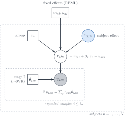
Figure 16: Stage II of imply (Meng et al. 2024) in this vignette’s notation. Subjects n are the independent units; their t_n repeated bulk samples i are correlated replicates. For gene g and type j, the subject reference r_{gjn} is a fixed group mean plus a subject random effect; the bulk mean mixes the subject references with the stage-I proportions \hat\theta_{j,ni}, held fixed. Stage III re-estimates the proportions by non-negative least squares with \boldsymbol{R}_n=[r_{gjn}].

imply estimates a reference per subject from that subject’s repeated bulk samples, then deconvolves those samples again with it (Meng et al. 2024). It assumes that the repeated samples of one subject, for example several brain regions or longitudinal draws, share one cell-type-specific profile and differ only in composition (p. 4). Single cells, or cell lines, enter only through the population signature of stage I. Below, n is the subject, i one of its t_n repeated samples, j the type and g the gene (the paper uses k for the type).

1. Stage I (p. 4). \nu-support vector regression of each sample on a population signature; negative estimates are set to zero and the rest renormalised, which gives \hat\theta_{j,ni}.

2. Stage II (pp. 4–5). For each gene, a linear mixed model with the stage-I proportions as covariates,

   \mathbb{E}(y_{g,ni})=\sum_j\bigl(m_{gj}+\beta_{gj}z_n+u_{gjn}\bigr)\hat\theta_{j,ni}, \tag{26}

   with z_n a binary group label, fixed effects m_{gj} (control mean) and \beta_{gj} (group difference), and a subject random effect u_{gjn}. It is fitted by penalised least squares with restricted maximum likelihood (REML), and the subject reference is r_{gjn}=\hat m_{gj}+z_n\hat\beta_{gj}+\hat u_{gjn} (p. 5): the best linear unbiased predictor of the subject’s profile. The covariance of u_{gjn} across types is not stated in the main text.

3. Stage III (p. 5). Non-negative least squares jointly over the samples of subject n, \min_{\boldsymbol{\Theta}_n\ge0}\lVert(\boldsymbol{R}_n\otimes\mathbf{I}_{t_n})\operatorname{vec}(\boldsymbol{\Theta}_n^{\top})-\operatorname{vec}(\boldsymbol{y}_n^{\top})\rVert_2, by quadratic programming.

Reading. Stage II is the reverse problem of Sec. 3 at the subject level: the composition is known, the profiles are random, and the BLUP returns them. It is the gene-wise analogue of DeCovarT’s Wiener filter read as a linear mixed model (LMM reading), with one random effect shared by the t_n repeated samples of a subject instead of one profile per bulk sample, and no gene–gene covariance. The stage-III objective equals \sum_i\lVert\boldsymbol{R}_n\boldsymbol{\theta}_{\cdot ni}-\boldsymbol{y}_{\cdot ni}\rVert^{2} under element-wise non-negativity, so the joint fit separates into one NNLS per sample with a shared \boldsymbol{R}_n (our remark). The same samples build \boldsymbol{R}_n and are deconvolved with it, and the stage-I proportions enter stage II as exact covariates: the data are used twice, and no interval is returned (our remark).

Perspective: a count mixed model (ours). The linear mixed model is the Gaussian member of rung 7. On counts, the natural extension is a negative-binomial mixed model with an identity link on the mixture mean, \mathbb{E}(y_{g,ni}\mid u)=s_{ni}\sum_j(m_{gj}+\beta_{gj}z_n+u_{gjn})\hat\theta_{j,ni} and \operatorname{Var}(y_{g,ni}\mid u)=\mathbb{E}+\mathbb{E}^{2}/\phi_g, with s_{ni} a library size, fitted by Laplace approximation as in glmmTMB-type software. The identity link keeps the physical sum of cells; a log link would mix logarithms (caveat 1 of Sec. 7). The mean must then stay positive, a constraint the solver has to enforce.

Ladder and errors in variables (Sec. 2.3, Sec. 2.2): rung 7 for the subject references (a Gaussian linear mixed model), rung 1 for the final proportions (NNLS with \boldsymbol{R}_n plugged in); the stage-I proportions are treated as exact; no interval.

Bayesian reference-based deconvolution

Bayesian methods put priors on the purified profiles, on the proportions, or on both, and report posterior summaries. They split by target: sample-level profiles (Sec. 4.1) or proportions (Sec. 4.2). A latent-profile Bayesian version of DeCovarT is derived in the Bayesian Wiener-filter vignette.

Cell-type-specific profiles

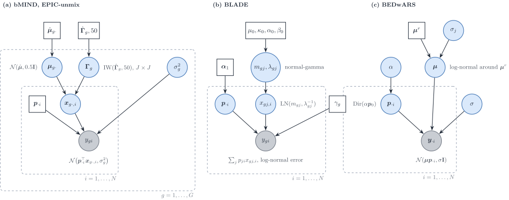
Figure 17: Bayesian models for cell-type-specific profiles, in this review’s notation. (a) bMIND and EPIC-unmix: for each gene, the sample-level profile across cell types is Gaussian with a J\times J covariance \boldsymbol{\Gamma}_g under an inverse-Wishart prior centred on single-cell estimates; proportions are fixed. (b) BLADE: log-normal profiles with a normal-gamma prior, Dirichlet proportions, linear mixing. (c) BEDwARS: a cohort-level signature drawn around a noisy reference, Dirichlet proportions, Gaussian residuals.

bMIND estimates sample-level profiles for proportions estimated beforehand (by NNLS or Bisque) (Wang et al. 2020). For gene g and subject i,

y_{gi}=\boldsymbol{p}_{\cdot i}^{\top}\boldsymbol{x}_{g\cdot,i}+e_{gi}, \qquad \boldsymbol{x}_{g\cdot,i}\sim\mathcal{N}_J(\boldsymbol{\mu}_{g\cdot},\boldsymbol{\Gamma}_g), \qquad e_{gi}\sim\mathcal{N}(0,\sigma_g^{2}), \tag{27}

with \boldsymbol{\mu}_{g\cdot}\sim\mathcal{N}(\hat{\boldsymbol{\mu}}_{g\cdot},0.5\mathbf{I}), \boldsymbol{\Gamma}_g\sim\mathrm{IW}(\hat{\boldsymbol{\Gamma}}_g,50) and a non-informative prior on \sigma_g^{2}; the hyperparameters come from single-cell or single-nucleus summary statistics. Sampling is by MCMC (MCMCglmm), gene by gene. Condition-specific means \boldsymbol{\mu}_g^{f} give tests of cell-type-specific differential expression. The authors note that the uncertainty of the estimated proportions is not propagated.

EPIC-unmix (Tang et al. 2025) keeps the bMIND model and adds a second, empirical-Bayes step: the prior is re-centred on the step-one posterior means and on their covariance across the target samples, with an increased number of degrees of freedom The target samples are therefore used twice. The bulk enters on the \log_2 scale, so the linear mixing of Eq. 27 is a mixing of logarithms, which is not the physical sum of cells (\log\sum_jp_jx_j\neq\sum_jp_j\log x_j).

BLADE estimates proportions and sample-level profiles jointly (Andrade Barbosa et al. 2021): y_{gi}=\sum_jp_{ji}x_{gj,i} plus a log-normal error, with x_{gj,i}\sim\mathrm{LN}(m_{gj},\lambda_{gj}^{-1}), a normal-gamma prior on (m_{gj},\lambda_{gj}) centred on the log-scale mean and variance of single-cell data, and \boldsymbol{p}_{\cdot i}\sim\mathrm{Dir}(\boldsymbol{\alpha}_1). The mixing is on the linear scale (TPM). Inference is collapsed variational, with hyperparameters chosen on a grid by likelihood. The model is diagonal: no covariance across genes or across types.

BEDwARS treats the reference itself as noisy (Ghaffari et al. 2023): y_{gi}=\sum_j\mu_{gj}p_{ji}+E_{gi}, \log\mu_{gj}\sim\log\mu^{r}_{gj}+\mathcal{N}(0,\sigma_j^{2}\log\mu^{r}_{gj}), \boldsymbol{p}_{\cdot i}\sim\mathrm{Dir}(\alpha\boldsymbol{p}_0), with half-Cauchy hyperpriors and Metropolis–Hastings chains. The signature is cohort-level: there is no sample-level profile. As written, the prior variance \sigma_j^{2}\log\mu^{r}_{gj} is not positive for reference values at or below one RPKM (our remark).

BayesPrism places a multinomial likelihood on bulk counts with a patient-derived single-cell prior and infers proportions and sample-level profiles jointly by Gibbs sampling (Chu et al. 2022). The multinomial is the Poisson measurement model conditioned on the library size (Sec. 1.1), so BayesPrism is the count-scale member of this family. When the reference is updated, the non-malignant profiles pooled across bulks deviate from the single-cell profiles by gene-wise fold changes with a weak, zero-mean log-normal prior (\sigma=2, pp. 5–6): a gene-wise random effect that absorbs platform factors, as \gamma_g does in RCTD (our reading). The read model has no overdispersion, and genes are coupled only through the multinomial total.

Table 5: Bayesian methods for cell-type-specific profiles. None models a G\times G gene–gene covariance.

Method	Bulk scale	Profile prior	Covariance	Proportions	Inference	Output
bMIND	linear (not stated)	\mathcal{N}(\boldsymbol{\mu}_g,\boldsymbol{\Gamma}_g)	IW on J\times J \boldsymbol{\Gamma}_g	fixed	MCMC	sample-level profiles
EPIC-unmix	\log_2	as bMIND, re-centred	IW on J\times J, empirical Bayes	fixed	MCMC, two steps	sample-level profiles
BLADE	linear (TPM)	log-normal, normal-gamma	none	Dirichlet	collapsed VI	proportions, sample-level profiles
BEDwARS	linear (RPKM)	log-normal around the reference	none	Dirichlet	MH chains	proportions, cohort signature
BayesPrism	counts	from single cells	none	Dirichlet	Gibbs	proportions, sample-level profiles
BLEND	counts	convex mixture of M_j observed references, Dirichlet weights	none stated; rank \le M_j-1 implied (our remark)	Dirichlet	Gibbs or EM-MAP	RNA fractions, per-sample references

The contrast with DeCovarT is the dimension of the covariance. bMIND and EPIC-unmix model how cell types covary for one gene across subjects; DeCovarT models how genes covary within one cell type. A separable covariance \operatorname{Cov}(\operatorname{vec}\boldsymbol{X}_i)=\boldsymbol{\Gamma}\otimes\boldsymbol{\Sigma} for the G\times J matrix of purified profiles would contain both as special cases (our remark); no reviewed method fits it.

BLEND: a per-sample mixture of references

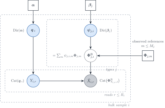
Figure 18: BLEND (Huang et al. 2024) in this vignette’s notation. Each bulk sample i draws RNA fractions \boldsymbol{q}_{\cdot i} and, for each type j, weights \boldsymbol{\psi}_{j,i} over the M_j observed references \boldsymbol{\Phi}_{j,m}; the sample’s reference for type j is their convex combination. Each read draws a type, then a gene from that type’s sample reference, so the gene counts are multinomial.

BLEND is the count member of this family with several references per type (Huang et al. 2024). Its generative model (p. 8) is latent Dirichlet allocation with per-sample topics. For bulk sample i with read depth R_i,

\boldsymbol{q}_{\cdot i}\sim\mathrm{Dir}(\boldsymbol{\alpha}), \qquad \boldsymbol{\psi}_{j,i}\sim\mathrm{Dir}(\boldsymbol{\beta}_j), \qquad \boldsymbol{y}_{\cdot i}\mid\boldsymbol{q}_{\cdot i},\{\boldsymbol{\psi}_{j,i}\} \sim\mathrm{Mult}\Bigl(R_i,\ \sum_jq_{ji}\,\boldsymbol{\Phi}^{\mathrm{B}}_{j,i}\Bigr), \qquad \boldsymbol{\Phi}^{\mathrm{B}}_{j,i}=\sum_{m=1}^{M_j}\psi_{j,i,m}\boldsymbol{\Phi}_{j,m}, \tag{28}

where the \boldsymbol{\Phi}_{j,m} are the observed references of type j, each a distribution over genes. The reference of type j in sample i thus lies in the convex hull of the observed references (p. 8). The multinomial collects the reads of steps (iii)–(v) of the paper, each drawn independently given the fractions and the weights (our rewriting).

• Inference (pp. 9–10). Gibbs sampling, after each read is given its reference source as an extra latent label, with all entries of \boldsymbol{\alpha} and \boldsymbol{\beta}_j set to 0.01; or EM for the maximum a posteriori estimate under the simplex constraints. On one bulk sample of 6,388 genes with nine references, the Gibbs sampler takes 36 minutes and EM-MAP 1.5 minutes (p. 10). The authors call these priors non-informative; a Dirichlet with concentrations 0.01 favours sparse weights, near the vertices of the simplex (our remark).
• Cell size (p. 10). \boldsymbol{q}_{\cdot i} are RNA fractions; cell fractions are p_{ji}=(q_{ji}/S_j)/\sum_{j'}(q_{j'i}/S_{j'}), with S_j given or estimated by average library sizes.
• Stated limits (p. 7). “Gene-gene correlation is ignored in BLEND for model simplicity”, and, although the posterior is available, “statistical inference for cellular fractions is not appropriate”.

Comparison with the Wiener filter. Both BLEND and DeCovarT’s latent-profile form (Wiener filter) return a profile per type and per bulk sample. BLEND restricts it to the hull of the observed references: at most M_j-1 free weights per type, on the scale of relative abundances, so a deviation that no reference shows cannot be expressed. The Wiener filter shrinks the bulk residual continuously onto each type along \boldsymbol{\Sigma}_j, can return any vector in \mathbb{R}^{G}, and has a closed-form posterior covariance (posterior covariance). Gene dependence is not absent from BLEND: across samples, \operatorname{Cov}(\boldsymbol{\Phi}^{\mathrm{B}}_{j,i})=\boldsymbol{\Phi}_j\operatorname{Cov}(\boldsymbol{\psi}_{j,i})\boldsymbol{\Phi}_j^{\top}, with \boldsymbol{\Phi}_j=[\boldsymbol{\Phi}_{j,1},\ldots,\boldsymbol{\Phi}_{j,M_j}], a gene–gene covariance of rank at most M_j-1 carried by the references (our remark). With a sample covariance of the M_j references plugged in as \boldsymbol{\Sigma}_j, the Wiener filter would be the Gaussian, continuous counterpart of that hull (our remark).

Ladder and errors in variables (Sec. 2.3, Sec. 2.2): rung 7, a multinomial given latent fractions and reference weights; the reference error is modelled only as a choice within the hull of the observed references; posterior summaries, which the authors do not use for inference.

Proportions

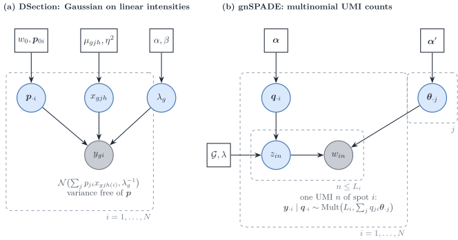
Figure 19: Bayesian estimation of proportions from continuous intensities or from counts. (a) DSection: Gaussian bulk on linear intensities with condition-specific type profiles, a gene-wise precision and an informative Dirichlet prior on the proportions. (b) gnSPADE: each UMI of a spot draws a type label and then a gene, so the spot counts are multinomial with a probability vector that mixes the type profiles; a gene network enters as a Markov random field on the labels.

DSection is the continuous, Gaussian route (Erkkilä et al. 2010): y_{gi}\sim\mathcal{N}\bigl(\sum_jp_{ji}x_{gjh(i)},\lambda_g^{-1}\bigr), with type profiles specific to the condition h(i) of sample i, x_{gjh}\sim\mathcal{N}(\mu_{gjh},\eta^{2}), \lambda_g\sim\mathrm{Gamma}(\alpha,\beta) and \boldsymbol{p}_{\cdot i}\sim\mathrm{Dir}(w_0\boldsymbol{p}_{0i}) centred on a prior guess of the proportions, which is needed for identifiability. Sampling is Gibbs for the profiles and the precision and Metropolis–Hastings with Dirichlet proposals for the proportions. The paper offers no log-normal option and recommends linear data. The variance depends on the gene but not on the proportions.

gnSPADE (Xie and Cui 2026) is the count route, and it is reference-free. Each UMI of spot i draws a label z\sim\mathrm{Mult}(\boldsymbol{q}_{\cdot i}) and then a gene from the profile of that label, so \boldsymbol{y}_{\cdot i}\mid\boldsymbol{q}_{\cdot i}\sim\mathrm{Mult}(L_i,\sum_jq_{ji}\boldsymbol{\theta}_{\cdot j}), with L_i the number of UMIs: latent Dirichlet allocation with a Markov random field over the labels built from a protein interaction network. Inference is collapsed Gibbs.

The two differ where the measurement model of Sec. 1 bites.

• Variance. In gnSPADE the variance is fixed by the mean (the multinomial is a Poisson measurement conditioned on the total). In DSection it is a free gene-wise constant that does not grow with the mean, which a UMI measurement contradicts.
• What the weights are. gnSPADE shares UMIs, so the label probabilities are transcript fractions \boldsymbol{q}_{\cdot i}; converting them to cell fractions needs S_j. DSection estimates whatever its reference scale encodes.
• Profile variability. Neither model has a type-level variability of profiles across samples beyond the prior of DSection; neither has a gene–gene covariance. The gene network of gnSPADE acts on labels, not on expression.

Semi-reference deconvolution: one unknown component

Semi-reference methods have references for J-1 types and estimate an unknown component, usually tumour, together with the proportions. With one component unknown, the convolution of univariate laws has to be written explicitly, and its tractability drives the choice of law.

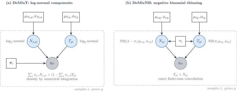
Figure 20: Two semi-reference convolutions of univariate components. (a) DeMixT: log-normal components mixed linearly on the raw scale; the density of the sum has no closed form and is integrated numerically. (b) DeMixNB: each component is a negative binomial whose mean is already scaled by its proportion; the density of the sum is an exact finite sum.

DeMix and DeMixT. DeMix mixes a tumour and one normal component; DeMixT adds a second normal component (Ahn et al. 2013; Wang et al. 2018):

y_{gi}=\pi_{1,i}N_{1,gi}+\pi_{2,i}N_{2,gi}+(1-\pi_{1,i}-\pi_{2,i})T_{gi}, \qquad N_{j,gi},T_{gi}\sim\log_2\text{-normal}. \tag{29}

The mixing is linear on the raw scale, and the density of a sum of log-normals has no closed form, so DeMixT integrates numerically (a double integral for three components). The normal-component parameters are plugged in from unmatched normal samples; the proportions and the tumour parameters are maximised by iterated conditional modes, gene and sample blocks in parallel. When the two normal means are close, the likelihood is flat in (\pi_1,\pi_2); a gene-set component-merging step first estimates the tumour proportion on genes where they agree. Genes are independent.

DeMixNB replaces the log-normal by a negative binomial for sparse counts (miRNA, spatial spots) (Montierth et al. 2025): T_{gi}\sim\mathrm{NB}(\pi_i\mu_{tg},\phi_{tg}), N_{gi}\sim\mathrm{NB}((1-\pi_i)\mu_{ng},\phi_{ng}) and y_{gi}=T_{gi}+N_{gi}, whose density is the finite sum \sum_{z=0}^{y}f_T(z)f_N(y-z). The proportions scale the means, not the dispersions. Read with Sec. 1, \mathrm{NB}(\pi\mu,\phi) is the binomial thinning of \mathrm{NB}(\mu,\phi): a Poisson measurement of a Gamma-distributed rate, with the rates mixed linearly (our remark). That makes DeMixNB the semi-reference model closest to a UMI measurement. Its \pi_i is a transcript fraction. The method is a preprint.

BayICE models \log(\text{count}+1) as Gaussian with mean \alpha_g+\sum_jw_{ji}\beta_{gj}+w_{0i}\beta_{g0}, a convex combination of type effects plus an unknown-class effect, with spike-and-slab priors on the type effects (marker selection with a Bayesian false discovery rate) and a Dirichlet prior on the weights (Tai et al. 2021). Inference is Gibbs with Metropolis–Hastings steps. The mixing is on the log scale, so it is a mean regression rather than a convolution, and the variances are gene-wise, not type-specific.

ISOpureR places a multinomial on the discretised tumour profile, with probability vector \alpha_i\boldsymbol{c}_i+\sum_r\omega_{ri}\boldsymbol{x}^{\mathrm{ref}}_r: the normal part is a convex combination of individual reference samples, the cancer profile \boldsymbol{c}_i is shrunk towards a cohort mean by a Dirichlet prior, and the estimate is a MAP by block coordinate descent (Anghel et al. 2015). Genes are coupled through the multinomial simplex; there is no overdispersion. Its \alpha_i is a fraction of transcripts.

Table 6: Semi-reference methods. The extension of DeCovarT to one unknown component is outlined in the extensions roadmap.

	DeMix, DeMixT	DeMixNB	BayICE	ISOpureR
Component law	\log_2-normal	negative binomial	Gaussian on \log(y+1)	multinomial, Dirichlet profiles
Mixing scale	raw	counts	log	probabilities
Convolution	numerical integration	exact finite sum	none (mean regression)	none (closed by thinning)
Inference	ICM, plug-in reference	ICM, L-BFGS-B, restarts	Gibbs and MH	MAP, coordinate descent
Genes	independent	independent	conditionally independent	coupled by the simplex
Proportion	mixing weight on raw scale	transcript fraction	weight on log scale	transcript fraction

Reference-free deconvolution with co-expression structure

Without a reference, deconvolution is a non-negative matrix factorisation \boldsymbol{Y}\approx\boldsymbol{\mu}\boldsymbol{P} with the columns of \boldsymbol{P} on the simplex. Three recent methods add gene–gene structure to that factorisation, in three different ways.

DSSC (Wang et al. 2024) fits the bulk and, in addition, the Gram matrices of genes and of samples :

\min_{\boldsymbol{\mu},\boldsymbol{P}\ge 0} \lVert\boldsymbol{Y}-\boldsymbol{\mu}\boldsymbol{P}\rVert_F^{2} +\lambda_1\lVert\boldsymbol{K}_N-\boldsymbol{P}^{\top}\boldsymbol{P}\rVert_F^{2} +\lambda_2\lVert\boldsymbol{K}_G-\boldsymbol{\mu}\boldsymbol{\mu}^{\top}\rVert_F^{2} +\lambda_c\lVert\boldsymbol{\mu}-\mathcal{T}(\boldsymbol{Y}_{\mathrm{sc}})\rVert_F^{2}, \tag{30}

where \boldsymbol{K}_G and \boldsymbol{K}_N are similarity kernels 1/(1+d) built from Pearson distances of the same bulk, and the last term optionally pulls the signature towards a transform \mathcal{T} of a single-cell reference. Multiplicative updates are run without the sum-to-one constraint and the proportions are normalised afterwards. The gene term matches \boldsymbol{\mu}\boldsymbol{\mu}^{\top} to a data similarity; expanded, it keeps the affinity part of a graph-Laplacian penalty and replaces its degree term by a quartic term, so it corresponds to no Gaussian Markov random field (our remark).

GSNMF+ (Li et al. 2025) regularises the rows of the signature with a kernel co-expression graph built on the bulk augmented by single-cell pseudo-bulks, and pulls marker rows towards the simplex vertices It states identifiability conditions (separability, or sufficiently scattered factors) and that the Frobenius loss is the Gaussian maximum-likelihood estimate. With a Euclidean distance its graph term would be \operatorname{tr}(\boldsymbol{\mu}^{\top}\boldsymbol{L}_G\boldsymbol{\mu}), the log-density of an intrinsic Gaussian Markov random field prior on the signature; with the cosine distance it uses, the term is quartic.

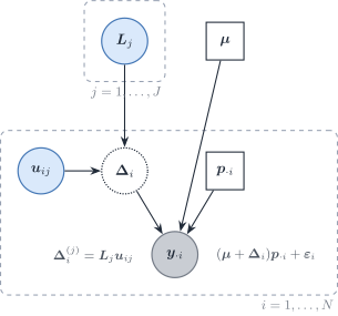
Figure 21: swCAM read as a probabilistic model (our reading, not the paper’s). The nuclear-norm penalty on the sample-specific deviations of type j is the MAP of a Gaussian factor model with loadings \boldsymbol{L}_j and sample scores \boldsymbol{u}_{ij}, which implies a low-rank gene–gene covariance within each cell type.

swCAM estimates sample-specific signatures (Chen et al. 2022). After convex analysis of mixtures has fixed \boldsymbol{\mu} and \boldsymbol{P}, it solves

\min_{\{\boldsymbol{\Delta}_i\}} \tfrac12\sum_i\lVert\boldsymbol{y}_{\cdot i}-(\boldsymbol{\mu}+\boldsymbol{\Delta}_i)\boldsymbol{p}_{\cdot i}\rVert_2^{2} +\lambda\sum_j\lVert\boldsymbol{T}_j\rVert_{*}, \tag{31}

where \boldsymbol{T}_j stacks the deviations of type j over samples and \lVert\cdot\rVert_* is the nuclear norm. The problem is convex for fixed \boldsymbol{\mu} and \boldsymbol{P} and is solved by ADMM. There is no co-expression graph. Because \lVert\boldsymbol{T}\rVert_*=\min_{\boldsymbol{A}\boldsymbol{B}^{\top}=\boldsymbol{T}}\tfrac12(\lVert\boldsymbol{A}\rVert_F^{2}+\lVert\boldsymbol{B}\rVert_F^{2}), the penalty is the MAP of a Gaussian factor model (Figure 21), which implies a low-rank gene–gene covariance within each type.

Three ways gene covariance enters deconvolution

1. Graph regularisation of a factorisation. A co-expression graph smooths the signature (GSNMF+). Its probabilistic reading is a Gaussian Markov random field prior on the signature, exact only for a Euclidean, quadratic penalty.
2. Similarity matching to the bulk itself. The Gram matrices of the factors are fitted to similarities computed from the same data (DSSC). The data are used twice, and no likelihood is implied.
3. Covariance in a likelihood, a moment equation or a prior. The gene–gene covariance of each type enters the bulk law: as a plug-in in DeCovarT, as moment equations in DECALS and MEAD, as the estimand in CSNet, and implicitly as a low-rank factor structure in swCAM. bMIND and EPIC-unmix belong here with the transposed object, a covariance across cell types.

All three reference-free methods use a squared Frobenius loss, that is a homoscedastic Gaussian likelihood, and therefore ignore the mean–variance relationship of counts (Sec. 1.1).

Synthesis

Table 7: Where second-order information enters each method. “Quadratic” and “linear” refer to the weight of a type’s variance in the bulk variance (p_{ji}^{2} for a random population profile, p_{ji} for independent cells).

Method	Bulk scale	Bulk variance as a function of \boldsymbol{p}	Gene–gene covariance	Type–type covariance	Reference uncertainty	Rung (Table 3)	Estimator
MuSiC	relative abundance	quadratic, diagonal	no	no	weights	2	weighted NNLS
SCDC	relative abundance	diagonal, clipped weights	no	no	no	2	weighted NNLS, ensemble
RNA-Sieve	counts / linear	linear, diagonal	no	no	noisy means	4 (composite)	MLE, Godambe
ReDeconv	linear (CLTS)	linear, diagonal	no	no	no	4	MLE
DWLS	linear	implied quadratic in the mean	no	no	no	2	weighted LS
deMixSC	relative abundance	fitted mean squared plus residual squared	no	no	no	2	iterated weighted NNLS
RCTD	counts	Poisson–log-normal	no	no	no	7	two-stage MLE
DeconV	counts	Poisson or negative binomial, plus a term quadratic in p_{ji} from the Gamma rate (our reading)	no	no	fitted prior	3	stochastic gradient (Pyro, clipped Adam)
DECALS	FPKM	quadratic	yes (moments)	no	no	6 (5 set aside)	OLS + sandwich
MEAD	linear	sandwich over dependent genes	yes (global)	no	yes	2 inside 6	estimating equations
DeCovarT	linear	quadratic	yes (plug-in, sparse)	no	bootstrap	5	MLE
CSNet	FPKM	quadratic	yes (estimand)	no	no	1 (reverse problem)	moments + thresholding
Unico	linear	\boldsymbol{p}^{\top}\boldsymbol{\Gamma}_g\boldsymbol{p}+\tau_g^{2}	no	yes (J\times J)	no	4 (reverse problem)	generalised method of moments
imply	not stated	through a subject random effect	no	not stated in the main text	subject-level BLUP	7, then 1	REML linear mixed model, then NNLS
bMIND, EPIC-unmix	linear / \log_2	\boldsymbol{p}^{\top}\boldsymbol{\Gamma}_g\boldsymbol{p}+\sigma_g^{2}	no	yes (J\times J)	prior	7	MCMC
BLADE	linear	quadratic, log-normal profiles	no	no	prior	7	collapsed VI
BayesPrism	counts	multinomial given latent profiles	no	no	prior	7	Gibbs
BLEND	counts	multinomial given latent reference weights	rank \le M_j-1, implicit (our remark)	no	convex hull of references	7	Gibbs or EM-MAP
BEDwARS	linear	constant	no	no	noisy reference prior	1	MH
DSection	linear	gene-wise, free of \boldsymbol{p}	no	no	prior	2	Gibbs–MH
DeMixT	raw	quadratic, log-normal components	no	no	plug-in	7	ICM
DeMixNB	counts	negative binomial	no	no	plug-in	3	ICM
swCAM	linear	constant	low rank (implicit)	no	no	1	ADMM

Caveats and defaults

1. Scale. Mixing is additive only on a linear scale. Methods that mix logarithms (BayICE, EPIC-unmix) estimate weights of a different, non-physical sum.
2. Cell versus RNA fractions. Count and topic models (ISOpureR, gnSPADE, DeMixNB, BayesPrism) and any fit on library-normalised bulk return transcript fractions; cell fractions need the cell sizes S_j (RNA-to-cell conversion).
3. Mean–variance relationship. A residual variance that does not grow with the mean (DSection, BEDwARS, NMF with a Frobenius loss, on rungs 1 and 2) contradicts the Poisson measurement of UMI counts, whose variance grows with the mean. Count likelihoods or explicit variance functions respect it (GLM view).
4. Linear or quadratic weights. Independent cells give a variance linear in the proportions (RNA-Sieve, ReDeconv); a random population profile gives a quadratic weight (MuSiC, DECALS, CSNet, DeCovarT). Single-cell references with one donor identify only the first (single-cell generative vignette).
5. Which covariance. G\times G within a type (DeCovarT, DECALS, CSNet) and J\times J within a gene (bMIND, EPIC-unmix, Unico) answer different questions; neither family fits both.
6. Data reuse. Empirical-Bayes re-centring on the target samples (EPIC-unmix), similarity graphs built from the bulk being factorised (DSSC, GSNMF+) and priors built from the same single-cell source as the benchmark bulk (BLADE group mode) inflate apparent accuracy.
7. Propagated uncertainty. Weighted moment estimators (MuSiC, SCDC, DWLS, deMixSC) return point estimates only (Sec. 2.3). Few methods propagate the uncertainty of the reference (RNA-Sieve, MEAD, DeCovarT’s reference bootstrap) or of the proportions into downstream profiles (bMIND and Unico do not).
8. Identifiability. Gene-wise scales with perfect markers (MEAD), collinear reference means (DeMixT), and reference-free factorisations without separability (GSNMF+) all leave the proportions unidentified, whatever the sample size.

References

Abbas, Alexander R., Kristen Wolslegel, Dhaya Seshasayee, Zora Modrusan, and Hilary F. Clark. 2009. ‘Deconvolution of Blood Microarray Data Identifies Cellular Activation Patterns in Systemic Lupus Erythematosus’. PloS One 4. https://doi.org/10.1371/journal.pone.0006098.

Agresti, Alan. 2015. Foundations of Linear and Generalized Linear Models. Wiley.

Ahn, Jaeil, Ying Yuan, Giovanni Parmigiani, et al. 2013. ‘DeMix: Deconvolution for Mixed Cancer Transcriptomes Using Raw Measured Data’. Bioinformatics (Oxford, England) 29. https://doi.org/10.1093/bioinformatics/btt301.

Andrade Barbosa, Bárbara, Saskia D. van Asten, Ji Won Oh, et al. 2021. ‘Bayesian Log-Normal Deconvolution for Enhanced in Silico Microdissection of Bulk Gene Expression Data’. Nature Communications 12 (1). https://doi.org/10.1038/s41467-021-26328-2.

Anghel, Catalina V, Gerald Quon, Syed Haider, et al. 2015. ‘ISOpureR: An R Implementation of a Computational Purification Algorithm of Mixed Tumour Profiles’. BMC Bioinformatics 16. https://doi.org/10.1186/s12859-015-0597-x.

Batardière, Bastien, Julien Chiquet, François Gindraud, and Mahendra Mariadassou. 2025. ‘Zero-Inflation in the Multivariate Poisson Lognormal Family’. Statistics and Computing 35 (6). https://doi.org/10.1007/s11222-025-10729-0.

Cable, Dylan M., Evan Murray, Luli S. Zou, et al. 2022. ‘Robust Decomposition of Cell Type Mixtures in Spatial Transcriptomics’. Nature Biotechnology 40 (4): 517–26. https://doi.org/10.1038/s41587-021-00830-w.

Cai, Biao, Emma Jingfei Zhang, Hongyu Li, Chang Su, and Hongyu Zhao. 2024. ‘Statistical Inference of Cell-Type Proportions Estimated from Bulk Expression Data’. Journal of the American Statistical Association 119 (548): 2521–32. https://doi.org/10.1080/01621459.2024.2382435.

Chen, Lulu, Chiung-Ting Wu, Chia-Hsiang Lin, et al. 2022. ‘swCAM: Estimation of Subtype-Specific Expressions in Individual Samples with Unsupervised Sample-Wise Deconvolution’. Bioinformatics 38 (5): 1403–10. https://doi.org/10.1093/bioinformatics/btab839.

Chen, Zeyuan Johnson, Elior Rahmani, and Eran Halperin. 2025. ‘Unico: A Unified Model for Cell-Type Resolution Genomics from Heterogeneous Omics Data’. Genome Biology 26 (1). https://doi.org/10.1186/s13059-025-03776-3.

Chiquet, Julien, Mahendra Mariadassou, and Stéphane Robin. 2018. Variational Inference for Sparse Network Reconstruction from Count Data. arXiv. https://doi.org/10.48550/arxiv.1806.03120.

Chiquet, Julien, Mahendra Mariadassou, and Stéphane Robin. 2021. ‘The Poisson-Lognormal Model as a Versatile Framework for the Joint Analysis of Species Abundances’. Frontiers in Ecology and Evolution 9. https://doi.org/10.3389/fevo.2021.588292.

Chu, Tinyi, Zhong Wang, Dana Pe’er, and Charles G. Danko. 2022. ‘Cell Type and Gene Expression Deconvolution with BayesPrism Enables Bayesian Integrative Analysis Across Bulk and Single-Cell RNA Sequencing in Oncology’. Nature Cancer 3 (4): 505–17. https://doi.org/10.1038/s43018-022-00356-3.

Dong, Meichen, Aatish Thennavan, Eugene Urrutia, et al. 2021. ‘SCDC: Bulk Gene Expression Deconvolution by Multiple Single-Cell RNA Sequencing References’. Briefings in Bioinformatics 22. https://doi.org/10.1093/bib/bbz166.

Erdmann-Pham, Dan D., Jonathan Fischer, Justin Hong, and Yun S. Song. 2021. ‘Likelihood-Based Deconvolution of Bulk Gene Expression Data Using Single-Cell References’. Genome Research 31 (10): 1794–806. https://doi.org/10.1101/gr.272344.120.

Erkkilä, Timo, Saara Lehmusvaara, Pekka Ruusuvuori, Tapio Visakorpi, Ilya Shmulevich, and Harri Lähdesmäki. 2010. ‘Probabilistic Analysis of Gene Expression Measurements from Heterogeneous Tissues’. Bioinformatics 26. https://doi.org/10.1093/bioinformatics/btq406.

Fan, Jiaxin, Yafei Lyu, Qihuang Zhang, Xuran Wang, Mingyao Li, and Rui Xiao. 2022. ‘MuSiC2: Cell-Type Deconvolution for Multi-Condition Bulk RNA-seq Data’. Briefings in Bioinformatics 23 (6). https://doi.org/10.1093/bib/bbac430.

Fang, Meichen, and Lior Pachter. 2025. Extrinsic Biological Stochasticity and Technical Noise Normalization of Single-Cell RNA Sequencing Data. bioRxiv preprint; bioRxiv. https://doi.org/10.1101/2025.05.11.653373.

Ghaffari, Saba, Kelly J. Bouchonville, Ehsan Saleh, Remington E. Schmidt, Steven M. Offer, and Saurabh Sinha. 2023. ‘BEDwARS: A Robust Bayesian Approach to Bulk Gene Expression Deconvolution with Noisy Reference Signatures’. Genome Biology 24 (1): 178. https://doi.org/10.1186/s13059-023-03007-7.

Godambe, V. P. 1960. ‘An Optimum Property of Regular Maximum Likelihood Estimation’. The Annals of Mathematical Statistics 31 (4): 1208–11. https://doi.org/10.1214/aoms/1177705693.

Guo, Shuai, Xiaoqian Liu, Xuesen Cheng, et al. 2023. ‘DeMixSC: A Deconvolution Framework That Uses Single-Cell Sequencing Plus a Small Benchmark Dataset for Improved Analysis of Cell-Type Ratios in Complex Tissue Samples’. bioRxiv, 2023.10.10.561733. https://doi.org/10.1101/2023.10.10.561733.

Gynter, Artur, Dimitri Meistermann, Harri Lähdesmäki, and Helena Kilpinen. 2023. DeconV: Probabilistic Cell Type Deconvolution from Bulk RNA-sequencing Data. bioRxiv. https://doi.org/10.1101/2023.12.07.570524.

Hansen, Lars Peter. 1982. ‘Large Sample Properties of Generalized Method of Moments Estimators’. Econometrica 50 (4): 1029–54. https://doi.org/10.2307/1912775.

Huang, Penghui, Manqi Cai, Chris McKennan, and Jiebiao Wang. 2024. BLEND: Probabilistic Cellular Deconvolution with Automated Reference Selection. bioRxiv. https://doi.org/10.1101/2024.08.02.606458.

Jew, Brandon, Marcus Alvarez, Elior Rahmani, et al. 2020. ‘Accurate Estimation of Cell Composition in Bulk Expression Through Robust Integration of Single-Cell Information’. Nature Communications 11. https://doi.org/10.1038/s41467-020-15816-6.

Lähdesmäki, Harri, llya Shmulevich, Valerie Dunmire, Olli Yli-Harja, and Wei Zhang. 2005. ‘In Silico Microdissection of Microarray Data from Heterogeneous Cell Populations’. BMC Bioinformatics 6. https://doi.org/10.1186/1471-2105-6-54.

Li, Shaoyu, Su Xu, Xue Wang, Nilüfer Ertekin-Taner, and Duan Chen. 2025. ‘An Augmented GSNMF Model for Complete Deconvolution of Bulk RNA-Seq Data’. Mathematical Biosciences and Engineering : MBE 22 (4): 988–1018. https://doi.org/10.3934/mbe.2025036.

Liu, Gan, Xiuqin Liu, and Liang Ma. 2022. ‘DecOT: Bulk Deconvolution with Optimal Transport Loss Using a Single-Cell Reference’. Frontiers in Genetics 13. https://doi.org/10.3389/fgene.2022.825896.

Lu, Songjian, Jiyuan Yang, Lei Yan, et al. 2025. ‘Transcriptome Size Matters for Single-Cell RNA-seq Normalization and Bulk Deconvolution’. Nature Communications 16 (1). https://doi.org/10.1038/s41467-025-56623-1.

Meng, Guanqun, Yue Pan, Wen Tang, et al. 2024. ‘Imply: Improving Cell-Type Deconvolution Accuracy Using Personalized Reference Profiles’. Genome Medicine 16 (1): 65. https://doi.org/10.1186/s13073-024-01338-z.

Montierth, Matthew D., Hao Yan, Liyang Xie, et al. 2025. Deconvolution of Sparse-count RNA Sequencing Data for Tumor Cells Using Embedded Negative Binomial Distributions. bioRxiv. https://doi.org/10.1101/2025.11.21.689822.

Nelder, J. A., and R. W. M. Wedderburn. 1972. ‘Generalized Linear Models’. Journal of the Royal Statistical Society. Series A (General) 135 (3): 370–84. https://doi.org/10.2307/2344614.

Sarkar, Abhishek, and Matthew Stephens. 2021. ‘Separating Measurement and Expression Models Clarifies Confusion in Single-Cell RNA Sequencing Analysis’. Nature Genetics 53 (6): 770–77. https://doi.org/10.1038/s41588-021-00873-4.

Shen-Orr, Shai S., Robert Tibshirani, Purvesh Khatri, et al. 2010. ‘Cell Type–Specific Gene Expression Differences in Complex Tissues’. Nature Methods 7. https://doi.org/10.1038/nmeth.1439.

Su, Chang, Jingfei Zhang, and Hongyu Zhao. 2024. ‘Estimating Cell-Type-Specific Gene Co-Expression Networks from Bulk Gene Expression Data with an Application to Alzheimer’s Disease’. Journal of the American Statistical Association 119 (546): 811–24. https://doi.org/10.1080/01621459.2023.2297467.

Tai, An-Shun, George C. Tseng, and Wen-Ping Hsieh. 2021. ‘BayICE: A Bayesian Hierarchical Model for Semireference-Based Deconvolution of Bulk Transcriptomic Data’. The Annals of Applied Statistics 15 (1). https://doi.org/10.1214/20-aoas1376.

Tang, Chenwei, Quan Sun, Xinyue Zeng, et al. 2025. ‘Cell Type-Specific Inference from Bulk RNA-Sequencing Data by Integrating Single-Cell Reference Profiles via EPIC-Unmix’. Genome Biology 26 (1): 395. https://doi.org/10.1186/s13059-025-03847-5.

Tsoucas, Daphne, Rui Dong, Haide Chen, Qian Zhu, Guoji Guo, and Guo-Cheng Yuan. 2019. ‘Accurate Estimation of Cell-Type Composition from Gene Expression Data’. Nature Communications 10. https://doi.org/10.1038/s41467-019-10802-z.

Wang, Chenqi, Yifan Lin, Shuchao Li, and Jinting Guan. 2024. ‘Deconvolution from Bulk Gene Expression by Leveraging Sample-Wise and Gene-Wise Similarities and Single-Cell RNA-Seq Data’. BMC Genomics 25 (1): 875. https://doi.org/10.1186/s12864-024-10728-x.

Wang, Jiebiao, Kathryn Roeder, and Bernie Devlin. 2020. Bayesian Estimation of Cell-Type-Specific Gene Expression Per Bulk Sample with Prior Derived from Single-Cell Data. openRxiv; openRxiv. https://doi.org/10.1101/2020.08.05.238949.

Wang, Xuran, Jihwan Park, Katalin Susztak, Nancy R. Zhang, and Mingyao Li. 2019. ‘Bulk Tissue Cell Type Deconvolution with Multi-Subject Single-Cell Expression Reference’. Nature Communications 10. https://doi.org/10.1038/s41467-018-08023-x.

Wang, Zeya, Shaolong Cao, Jeffrey S. Morris, et al. 2018. ‘Transcriptome Deconvolution of Heterogeneous Tumor Samples with Immune Infiltration’. iScience 9. https://doi.org/10.1016/j.isci.2018.10.028.

Xie, Aoqi, and Yuehua Cui. 2026. ‘gnSPADE: Incorporating Gene Network Structures Enhances Reference-Free Deconvolution in Spatial Transcriptomics’. Advanced Intelligent Systems 8 (4): e202500639. https://doi.org/10.1002/aisy.202500639.

Xie, Dongyue, Lin Gui, and Jingshu Wang. 2026. ‘Statistical Inference for Cell Type Deconvolution’. Journal of the Royal Statistical Society Series B: Statistical Methodology 88 (4): 1449–68. https://doi.org/10.1093/jrsssb/qkag054.