§2.4 Single-cell scenario: four cell types in two lineages (G = 20 or 200, J = 4)

library(DeCovarT)

The bivariate toy and the covariance-driven scenario use a population reference: every cell type is one purified Gaussian profile, and the bulk is their convolution. This scenario uses a single-cell reference: the bulk is the sum of n_i cells, each drawn from the law of its type, and DeCovarT fits the single-cell model with its two scales profiled out (single-cell model). The J=4 cell types form two lineages, types 1–2 and types 3–4, so every type has a close sibling and a distant cousin. Construction, benchmark and plot books live in one script, scripts/fig05_single_cell_hierarchical.R (seed 20261024).

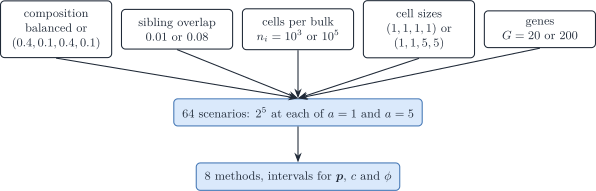
Figure 1: Single-cell factorial. Six crossed factors with two levels each give 64 scenarios: five design factors, crossed with the platform scale a = 1 or 5, which tests the scale assumption of RNA-Sieve. Every scenario is analysed by eight methods.

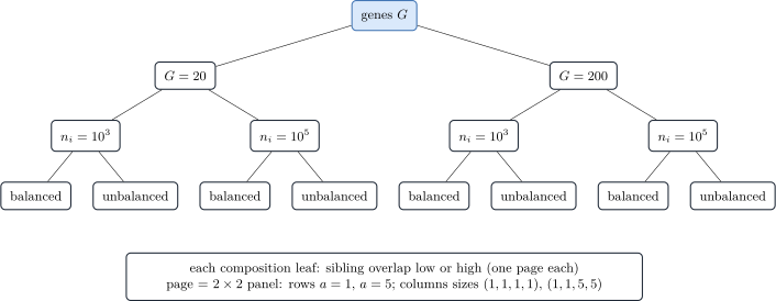
Figure 2: Order of the plot books. Pages nest the number of genes, the number of cells per bulk, the composition and the sibling overlap; inside each page, a 2-by-2 panel crosses the platform scale (rows) with the cell sizes (columns). Every cell of the grid is simulated.

Generative model

The generator is the single-cell model itself (cell size in the covariance). For bulk i,

\boldsymbol m_{\cdot i}\sim\operatorname{Multinomial}(n_i,\boldsymbol p), \qquad \boldsymbol T_{ji}\sim\mathcal N_G\bigl(m_{ji}S_j\boldsymbol\theta_{\cdot j},\; m_{ji}S_j^{2}\boldsymbol\Sigma^{\theta}_j\bigr), \qquad \boldsymbol y_{\cdot i}=a\sum_j\boldsymbol T_{ji}, \tag{1}

where \boldsymbol\theta_{\cdot j} is the expression profile of a cell of unit size, S_j the cell size of type j and a the platform scale. The estimand is the realised cell fraction \boldsymbol m_{\cdot i}/n_i, not \boldsymbol p (simulate_bulk_from_cells() returns it as p_realised).

A cell S_j times larger is S_j times larger in every gene, so the size multiplies the mean by S_j and the covariance by S_j^{2} (rescale_single_cell_moments()). Two consequences:

the overlap between two types of equal size does not depend on that size, so cell size only moves the lineages apart and reweights the bulk;
in transcript units the covariance of a cell is S_j\boldsymbol\Sigma^{\theta}_j, which is the form of the transcript_raw reference.

DeCovarT is fitted with the cellular_raw reference: cell fractions, known cell sizes and raw covariances.

Mean signature

One mean signature per gene count G\in\{20,200\} is built by generate_mean_signature_matrix(target_gram = R, nonnegative = TRUE) (mean signature construction), with mean scale 10 and the target Gram

R= \begin{pmatrix} 1 & 0.8 & 0.3 & 0.3\\ 0.8 & 1 & 0.3 & 0.3\\ 0.3 & 0.3 & 1 & 0.8\\ 0.3 & 0.3 & 0.8 & 1 \end{pmatrix}. \tag{2}

The cosine between lineages is 0.3, not 0.1. With non-negative means, the expression of a gene in the other lineage is then about 13\% of its main level; at a cosine of 0.1 it would be about 4\%, close to disjoint marker blocks, and the scenario would reduce to marker-gene deconvolution. Every gene is expressed in all four types.

Lineage networks

Each lineage has one skeleton, shared exactly by its two siblings:

Table 1: Graph of each cell type.

Type	Lineage	Skeleton
celltype_1	1	stochastic block model, three blocks of equal size
celltype_2	1	the same skeleton as celltype_1
celltype_3	2	scale-free (Barabási–Albert, `power = 1`)
celltype_4	2	the same skeleton as celltype_3

The blocks are contiguous in gene order (block_sizes of generate_random_network_skeleton()), with p_{\mathrm{within}}=0.25 and p_{\mathrm{between}}=0.01. Signed weights are drawn once per lineage by assign_iid_signed_weights() (half inhibitory, magnitude 0.3); each sibling then flips the sign of a random 5\% of the edges, so the two siblings differ only by their edge weights. With independent signs the sibling covariances differ so much at G=200 that a sibling overlap of 0.08 cannot be reached (at most 0.013; 0.030 with 20\% flips). Precisions are completed by build_normalised_precision() with a fixed spectral shift of 0.2 (GGM networks).

Sibling overlap

One global covariance scale per gene count and overlap target is chosen by scale_covariances_to_overlap(pairs = rbind(c(1, 2), c(3, 4))), so that the mean overlap of the two sibling pairs is 0.01 or 0.08 at the balanced composition. Calibrating on all six pairs would let the four nearly separated between-lineage pairs dilute the target. The scale is calibrated once on equal cell sizes and reused for unequal sizes, since the sibling overlap does not depend on a common size. In the dry run the realised mean of the two sibling pairs is 0.009 to 0.081. The two pairs differ (from 0.0005 to 0.149), because the block model and the scale-free graph give the two lineages different covariances. The overlaps are identical for equal and unequal sizes, and between-lineage overlaps stay at or below 0.001 (Monte Carlo estimates, 10^4 draws per type).

Factorial design

Table 2: Single-cell factorial (64 scenarios).

Factor	Levels
Composition \boldsymbol p	balanced (1/4,1/4,1/4,1/4); unbalanced within each lineage (0.4,0.1,0.4,0.1)
Sibling overlap	0.01; 0.08
Cells per bulk n_i	10^{3}; 10^{5}
Cell sizes \boldsymbol S	(1,1,1,1); (1,1,5,5)
Genes G	20; 200
Platform scale a	1; 5
Crossed scenarios	2^{6}=\mathbf{64}

Cells per bulk. With n_i\ge10^{3} the rarest type counts about 100 cells, so the multinomial draw does not leave a type empty.
Genes. The maximum-likelihood variance scale \hat\phi is biased down by about (G-J)/G, that is 0.8 at G=20 and 0.98 at G=200; the REML calibration corrects it (REML).
Platform scale. Rescaling the bulk by a rescales \hat c by a and \hat\phi by a^{2}, leaves \hat{\boldsymbol p} unchanged, and shifts the profile log-likelihood by -G\log a (scale equivariance), so the estimates of \boldsymbol p should agree between a=1 and a=5, which the crossed a=1 half checks numerically. It also tests RNA-Sieve, whose mean and variance share one scale.

Scenario identifiers read S{row}_{Ba|Un}_{O1|O8}_n{1e3|1e5}_{Se|Sl}_G{20|200}_a{1|5}, for example S1_Ba_O1_n1e3_Se_G20_a1.

# The design takes about a minute (overlap calibration by Sobol Monte
# Carlo for each gene count and target).
benchmark <- readRDS("output/fig05/fig05_benchmark.rds")
benchmark$config |>
  dplyr::select(
    ID, proportions, overlap_target, sibling_overlap, n_cells,
    cell_size_label, n_genes, platform_scale
  )

Inference

Every method is scored on the same simulated bulks, with all genes (no feature selection).

Table 3: Methods of the single-cell benchmark.

Method	Function or code	Input	Intervals
`lsei`	`deconvolute_ratios_deconrnaseq()`	true means	none
NNLS	`deconvolute_ratios_nnls()`	true means	none
RLM	`deconvolute_ratios_rlm()`	true means	none
CIBERSORT	`deconvolute_ratios_cibersort()`	true means	none
Newton–Raphson	`deconvolute_single_cell(optimiser = "newton")`	true moments, known sizes	Wald, ILR, ILR-REML, profile, profile-REML, oracle
L-BFGS-B	`deconvolute_single_cell(optimiser = "lbfgsb")`	true moments, known sizes	Wald, ILR, ILR-REML
Firth	`fit_firth_single_cell()`	true moments, known sizes	Wald, Wald-REML, ILR, ILR-REML
MEAD	`MEAD::MEAD()` (GitHub, commit `d66fa10`)	reference panel, cohort of N bulks	native sandwich interval
RNA-Sieve	`rnasieve` 0.1.4 (Python)	reference panel, cohort of N bulks	released, Fisher and Godambe
ReDeconv	`redeconv` 1.2.1 (Python)	true means and standard deviations	none

lsei and NNLS. The scale c=a\,n_i of a single-cell bulk is unknown, so lsei, which fixes it at one, is misspecified here. NNLS followed by renormalisation is the same least squares with a free scale (\boldsymbol\beta=c\boldsymbol p); it is also the starting point of DeCovarT and RNA-Sieve. RLM is the robust linear model of Monaco et al., renormalised.
DeCovarT. Newton–Raphson and L-BFGS-B maximise the same profile log-likelihood; L-BFGS-B works on the closure chart \boldsymbol p=\boldsymbol w/\mathbf1^{\top}\boldsymbol w, \boldsymbol w\ge0 (L-BFGS-B). Bootstraps refit with the optimiser of the estimate. A boundary estimate (one, two or up to J-1 zero proportions: a face, an edge or a vertex) has no Wald or ILR interval, for the fractions or the scales, so their coverage for L-BFGS-B is over interior estimates; n_boundary gives the count. Profile intervals refit from the bulk and are reported under Newton–Raphson only.
Second-generation methods follow the protocol of the covariance-driven scenario. MEAD and RNA-Sieve read a reference panel of R individuals and 20 cells per type and individual, drawn by simulate_reference_replicates() with its own seed, independent of the bulks.
- MEAD rescales every reference cell to a unit total, so its proportions are transcript fractions q_j=p_jS_j/\sum_kp_kS_k; with \boldsymbol S=(1,1,5,5) they differ from the cell fractions. Its intervals are scored against both.
- RNA-Sieve’s released interval code returns [0,1] when its averaged Hessian is ill-conditioned (version 0.1.4, stats.py, lines 224 and 234). The runner also returns the two intervals of the paper, recomputed on all genes: Fisher, \boldsymbol B^{-1}/G, and Godambe, \boldsymbol H^{-1}\boldsymbol B\boldsymbol H^{-\top}/G, with \alpha_K=1-\sum_{k<K}\alpha_k. In the dry run (N=5), averaged over the 132 scenario and cell-type pairs, the released interval has mean width 0.91 (coverage 1), the Godambe interval 0.36 (coverage 0.97) and the Fisher interval 0.002 (coverage 0.02). The per-gene scores vary far more than the Hessian predicts, since RNA-Sieve’s model is not the generator here, so only the sandwich is calibrated.
- DECALS has no public implementation and is not run.

Interval constructions

The menu is that of the single-cell inference article:

Interval	Construction
`wald`	delta method on \boldsymbol p from the Schur-complement information
`ilr`	Wald in ILR coordinates mapped back to the simplex
`profile`	likelihood-ratio inversion with c and \phi profiled out
`*_reml`	REML calibration with \nu=G-J: Student quantiles and \hat\phi rescaled by G/\nu
`oracle`	\hat p_j plus or minus the Wald half-width at the true composition

Wald and ILR intervals also cover the two scales, c=a\,n_i and \phi=a^{2}n_i (rows mean_scale and variance_scale of the interval table), and the platform scale a=\phi/c and the cell count n=c^{2}/\phi (rows platform_scale_a and cell_count_n), against their true values. The intervals of a and n are formed on the log scale, so both bounds are positive; \hat n is a number of cells here only because a is known to the generator. Coverage is reported with a Wilson Monte Carlo interval (Morris et al. 2019).

Run size

Table 5: Run-size constants at the top of scripts/fig05_single_cell_hierarchical.R.

Constant	Meaning	Value
`N_REPLICATES`	Monte Carlo bulks per scenario, N	200
`N_REFERENCE`	individuals of the reference panel, R (MEAD and RNA-Sieve)	200
`CORES`	workers for the N bulks of a scenario; the three figure scripts run at the same time	a third of half the cores (14 of 88)
`POSTPROCESS_ONLY`	`TRUE` redraws the figures from the saved benchmark	`FALSE`

The parametric bootstrap is not run: the moments of a scenario are fixed, so coverage is measured over its N bulks. Parallel workers load the installed DeCovarT, so run devtools::install() before a parallel run.

benchmark <- readRDS("output/fig05/fig05_benchmark.rds")
# Coverage of the composition and of the two scales.
dplyr::select(
  benchmark$intervals,
  ID, algorithm, ci_method, parameter, coverage, coverage_lower,
  coverage_upper, mean_width
)

Visualisations

output/fig05/fig05_benchmark.rds holds the run settings, the design, the true moments (theta_true) and every metric table; output/fig05/fig05_plot_data.rds holds, for each figure file stem, the data handed to its plot function.

source("scripts/visualisation/load_visualisation.R")
plot_data <- readRDS("output/fig05/fig05_plot_data.rds")
names(plot_data)
render_figure_from_data("ci_width_forest", plot_data, "output/fig05")

The books follow those of the covariance-driven scenario, with these changes:

pages follow Fig. 2: G, then n_i, the composition and the sibling overlap; each page is a 2\times2 panel with the platform scale in rows and the cell sizes in columns;
log-likelihood surfaces are drawn on the two within-lineage balances, 1\mid2 and 3\mid4, with the between-lineage balance held at its true value, each panel zoomed on its own peak;
CIBERSORT is left out of the RMSE and Aitchison heatmaps and of the RMSE dot book, where its large error squeezed the shared colour scale;
the scenario descriptors add n_i, G and the cell-size ratio;
the forests add the REML-calibrated ILR and profile intervals, and performance_visualisations/ci_width_forest_nuisance.pdf gives the intervals of c, \phi, a and n on \log_{10} axes;
performance_visualisations/nuisance_scale_ratio.pdf shows \hat c/c and \hat\phi/\phi against the number of genes and of cells, with the REML-rescaled \hat\phi\,G/(G-J).

Caveats

Gaussian cells. A sum of Gaussian cells is exactly Gaussian at any n_i, so the central-limit argument behind the bulk model is not itself tested; a count layer would be needed for that.
Negative values. Between 21\% and 29\% of the simulated single-cell values are negative. The reference panels of MEAD and RNA-Sieve receive them as such.
Per-cell overlap and bulk precision. The sibling overlap describes the reference; the precision of a bulk also grows with n_i, which the expected Wald standard error reported with each scenario captures.

References

Morris, Tim P., Ian R. White, and Michael J. Crowther. 2019. ‘Using Simulation Studies to Evaluate Statistical Methods’. Statistics in Medicine 38 (11): 2074–102. https://doi.org/10.1002/sim.8086.