This article is the bivariate Gaussian-convolution toy of the methods paper (G=2, J=2). It isolates gene–gene correlation from mean separation. The factorial grid and ADEMP pipeline live in a single script, scripts/fig02_bivariate_toy.R. Scenario builders (build_bivariate_scenario_config(), bivariate_toy_deconvolution_functions()) sit at the top of that file. Sourcing the script from a vignette or from a temp copy in tests defines those functions without launching the 972-scenario pipeline.
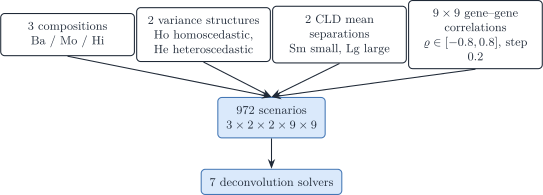
Figure 1: Bivariate toy factorial design: three compositions, two variance structures, two CLD mean separations, a 9-by-9 gene-gene correlation grid, and seven solvers (3 x 2 x 2 x 9 x 9 = 972 scenarios).
Figure 2: Hierarchical reading of the same factorial: small versus large CLD, then homoscedastic versus heteroscedastic variances, then balanced / moderately unbalanced / highly unbalanced compositions (2 x 2 x 3 = 12 meta-scenarios). Each leaf is crossed with the 9-by-9 gene-gene correlation grid.
Generative model
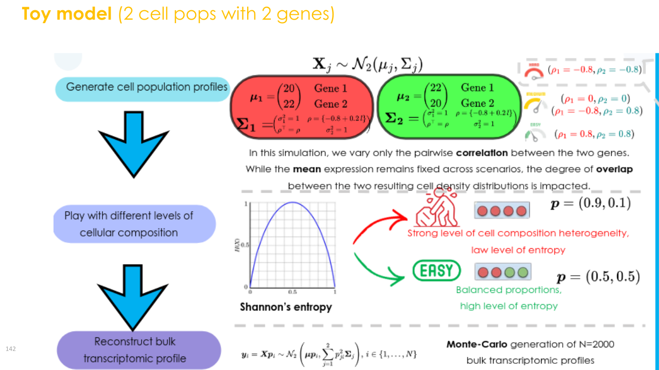
With p_1+p_2=1, only one free ILR coordinate is estimated (see derivatives under simplex transforms). Even when mean profiles are similar, gene–gene correlation can degrade mean-only solvers, and is partly recovered once \boldsymbol{\Sigma}(\boldsymbol{p})=\sum_j p_j^2\boldsymbol{\Sigma}_j enters the likelihood.
(a) Hyperparameter grid used in the bivariate manuscript study: two centroid geometries, balanced versus unbalanced \boldsymbol{p}, a gene–gene correlation sweep, and the first-generation plus DeCovarT solvers.
(b) AI-generated 2D density of the two-gene mixture while only the pairwise correlation changes, at fixed means, marginal variances, and composition. The ggplot panel below recomputes the same contrast and annotates MixSim overlap.
Figure 3: Factorial design (left) and correlation-only 2D densities (right) for the bivariate toy. {#fig-toy-design}
CLD is centroid (mean-profile) Euclidean separation \lVert\boldsymbol{\mu}_{\cdot 1}-\boldsymbol{\mu}_{\cdot 2}\rVert_2, not an Aitchison distance; see the descriptor notes. Small CLD uses \boldsymbol{\mu}_{\cdot 1}=(20,22), \boldsymbol{\mu}_{\cdot 2}=(22,20) (d=2\sqrt{2}\approx 2.83, cosine \approx 0.995). Large CLD uses (20,40) and (40,20) (d=20\sqrt{2}\approx 28.3, cosine 0.8).
Scenario ID
Each row is labelled B{index}_{variance}_{composition}_{CLD}. The index is the factorial row number (1–972). Example: B1_Ho_Ba_Sm is the first row, homoscedastic, balanced proportions, small CLD.
Every result of the run is in output/fig02/fig02_benchmark.rds, a list keyed by the scenario ID: meta (seed, N, B, date, git commit, session), config (the design grid without the true moments), theta_true (convolution parameters per ID), descriptors (geometry, MixSim BarOmega, Hellinger, Jeffreys), regression and monte_carlo (composition and ADEMP blocks of compute_benchmark_metrics()), optimisation (one row per replicate \times algorithm \times scenario, with the estimates, convergence, KKT residual, elapsed time and memory), intervals (coverage and width of every interval construction) and data (the simulated bulks and their targets).
Mean-only lsei and NNLS do not maximise the convolution likelihood, so no interval is computed for them.
For J=2 the free coordinate is p_1\in(0,1). The listing below evaluates \ell_{\boldsymbol{y}\mid\boldsymbol{\zeta}}(p_1,1-p_1) on one bulk draw. It is not executed during R CMD build: Quarto’s Windows CLI starts a new R process that cannot see the temporary library (quarto-r#217). The same likelihood path is checked in tests/testthat/.
set.seed(20260828)rho<-0.6R<-matrix(c(1, rho, rho, 1), nrow =2)Sigma<-array(c(R, R), dim =c(2, 2, 2))dimnames(Sigma)<-list(rownames(mu_small),rownames(mu_small),colnames(mu_small))y_one<-DeCovarT::simulate_bulk_mixture(mu_small,Sigma, p =p_bal, n =1)$Y[, 1]p1_grid<-seq(0.02, 0.98, by =0.01)ll_grid<-vapply(p1_grid,function(p1){DeCovarT::loglik_multivariate(c(p1, 1-p1), y_one, mu_small, Sigma)},numeric(1))ll_df<-data.frame(p1 =p1_grid, loglik =ll_grid)ggplot2::ggplot(ll_df, ggplot2::aes(x =p1, y =loglik))+ggplot2::geom_line(colour ="#1B4F72", linewidth =0.8)+ggplot2::geom_vline( xintercept =0.5, linetype ="dashed", colour ="grey30")+ggplot2::labs( x ="p1 (p2 = 1 - p1)", y ="Log-likelihood")+ggplot2::theme_bw(base_size =11)
Dropped from the figure. Marquardt–Levenberg, projected gradient and simulated annealing remain in the package but leave the benchmark. CIBERSORT is not run at G=2: its \nu-SVR regresses the G bulk values on the J signatures, so two genes give two observations for two coefficients and an intercept. The second-generation methods (MEAD, RNA-Sieve, ReDeconv, DECALS) are left to the covariance-driven scenario, since a two-gene reference cannot carry their reference estimation.
NNLS followed by renormalisation is least squares on the simplex with a free scale (\boldsymbol\beta=c\boldsymbol p, c=\mathbf 1^{\top}\boldsymbol\beta); lsei fixes c=1. The two agree only when \hat c=1. On 500 bulks of this design the largest coordinate difference has median 0.002 and 95th percentile 0.015, and the fitted scale has standard deviation 0.03 around 1: close, but not identical. Both are run: lsei keeps the sum-to-one equality and the bounds at every iteration, NNLS renormalises a free-scale fit. A robust linear model is not run on two genes.
The interval constructions are those of population inference: wald (delta method on \boldsymbol p), ilr (Wald in ILR coordinates mapped back), profile (likelihood-ratio inversion) and oracle (\hat p_j plus or minus the Wald half-width at \boldsymbol p^{\star}). The parametric bootstrap (bootstrap_decovart()) is not run here: the moments of a scenario are fixed, so coverage is measured over its N bulks, and N\times B refits per solver dominated the run time. Performance is summarised with the ADEMP framework (Morris et al. 2019): bias, RMSE, coverage of each interval construction (Wilson intervals on the coverage rate), width, SE/SD, and optimiser failure rate.
The run size is hard-coded at the top of the script: N_REPLICATES (N=200), CORES (workers for the N bulks of a scenario: a third of half the cores, 14 of 88, since the three figure scripts run at the same time; parallel workers load the installed package) and POSTPROCESS_ONLY (TRUE redraws only).
config on the in-memory benchmark still carries Shannon entropy of \boldsymbol{p} and MixSim overlap for tests.
Visualisations
Figures are drawn from output/fig02/fig02_plot_data.rds, a list keyed by figure file stem that holds the data handed to each plot function, so any figure can be redrawn without the benchmark:
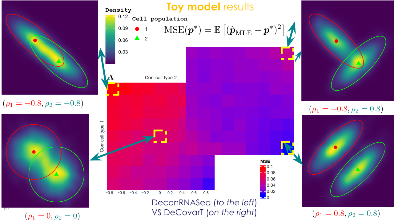
Density and performance books share the four correlation corners (\varrho_1,\varrho_2)\in\{(0,0),(-0.8,-0.8),(0.8,0.8),(-0.8,0.8)\} and the twelve meta-scenarios (CLD \times variance \times composition). Every log-likelihood panel uses the same axes and the same fill, \log_{10}(L/\max L) on [-10,0], with one legend per page: white diamond at \boldsymbol p^{\star}, red point at the MLE (observed surface) or at the Monte Carlo mean of \hat{\boldsymbol p} (expected surface, whose maximiser is \boldsymbol p^{\star} exactly by the information inequality).
The Q-Q books assess the Wald approximation only; the profile intervals do not rely on it. Squaring a whitened value of -30 gives D^2=900, so the \chi^2 book uses \log_{10} axes.
The Hellinger distance \lVert\sqrt{\hat{\boldsymbol p}_A}-\sqrt{\hat{\boldsymbol p}_B}\rVert_2/\sqrt2 replaces 1-r for the Pearson correlation: it measures agreement rather than co-movement, it is Euclidean in \sqrt{\boldsymbol p} as Ward’s criterion requires, and it is defined at exact zeros, where the Aitchison distance is not.
The KS normality lollipops and the MAE heatmaps were dropped: the Q-Q books and the RMSE heatmaps carry the same information.
Tip 1: Other one-sample log-likelihood slices (not drawn)
The current loglik_rgl.pdf holds the two mean profiles fixed and varies only \boldsymbol{p} (or its ILR coordinate). White diamonds mark p^{\star} and red circles the numerical MLE. Expected log-likelihood surfaces \mathbb{E}_{\boldsymbol{y}\mid\boldsymbol{p}^{\star}}[\ell(\boldsymbol{p};\boldsymbol{y})] are drawn separately as loglik_expected_surface_p.pdf and loglik_expected_ilr_profile.pdf (not overlaid on the one-draw books). Useful alternatives, left as outlook:
Hold \boldsymbol{p}^{\star} fixed and vary one column of \boldsymbol{\mu} (a mean-shift slice) to show how centroid collision flattens \ell.
Hold \boldsymbol{p}^{\star} and \boldsymbol{\mu} fixed and vary one correlation \varrho_j, so the surface is a covariance diagnostic rather than a mixing-weight diagnostic.
Overlay several independent bulk draws as translucent surfaces to display sampling variability of \ell(\boldsymbol{p};\boldsymbol{y}).
Likelihood geometry and solver behaviour
Note
The numbers in this section come from the archived run of output/archives/fig02/ (Wald intervals only), which still included NNLS, gradient, simulated annealing, Marquardt–Levenberg and the earlier L-BFGS-B that renormalised a box-constrained fit. They will be replaced by those of the production run; the mechanisms do not depend on the solver list.
The factorial heatmaps remain the right design summary: large CLD and \varrho_j=0 make the mean map injective, so every solver is accurate; small CLD plus aligned correlations flatten the mean residual and raise RMSE off the diagonal \varrho_1=\varrho_2. That saddle is a statement about identifiability of \boldsymbol{\mu}\boldsymbol{p}, not about which numerical method is used. The pack in output/fig02/mle_explanation/ (scenario descriptors, ILR profiles evaluated at \boldsymbol{y}=\boldsymbol{\mu}\boldsymbol{p}^{\star}, expected-Fisher Wald standard errors, and Newton versus Marquardt forests) is what separates three mechanisms that the heatmaps mix: the shape of \ell(\boldsymbol{p};\boldsymbol{y}), the surrogate each solver actually minimises, and the chart / stopping rule that walks that surrogate.
What is being optimised
Mean-only NNLS and DeconRNASeq (lsei in limSolve) minimise a convex quadratic (\boldsymbol{y}-\boldsymbol{\mu}\boldsymbol{p})^{\top}
(\boldsymbol{y}-\boldsymbol{\mu}\boldsymbol{p}) on the simplex (Dessole et al. 2023; Gong and Szustakowski 2013; Soetaert et al. 2026). For a convex objective a local minimiser is global (Boyd et al. 2004, ch. 4), so those fits are unique solutions of the least-squares problem. They are not maximisers of the convolution log-likelihood: \boldsymbol{\Sigma}(\boldsymbol{p}) never enters the quadratic. When \boldsymbol{\mu}_{\cdot 1} and \boldsymbol{\mu}_{\cdot 2} are close, that quadratic is a ridge along the simplex. A strictly feasible QP with bound constraints then has vertices as KKT candidates, which is why mean-only fits pile up at (1,0) and (0,1) whenever the residual is uninformative. Simulated annealing explores the same non-concave \ell as DeCovarT but without curvature, so it is a robustness check, not an MLE.
The convolution solvers maximise the Gaussian-convolution log-likelihood of the MLE properties article (that article is pkgdown-only; this vignette is the CRAN-shipped companion). None of them inherits Boyd’s global certificate, because that likelihood is not concave. They differ in coordinates and damping:
L-BFGS-B (stats::optim) runs limited-memory BFGS on the closure chart \boldsymbol p=\boldsymbol w/\mathbf 1^{\top}\boldsymbol w with the box \boldsymbol w\ge0(Byrd et al. 1995; Zhu et al. 1997) (closure chart). The objective is the convolution log-likelihood itself, the box KKT points are exactly the simplex KKT points, and exact zeros are reachable. The archived version instead fitted a box-constrained surrogate and renormalised it, so its faces were not stationary points of \ell (KKT residual about 0.1).
Newton-Raphson (stats::nlminb) and Marquardt-Levenberg (marqLevAlg; (Philipps et al. 2023, 2021)) work in ILR coordinates, so the walk stays in the relative interior until a coordinate diverges. Newton uses the analytic Hessian. Marquardt adds a Levenberg damping term so that the working matrix stays positive definite (Marquardt 1963) even when the Hessian of \ell is indefinite, and stops on the relative-distance-to-maximum (RDM) criterion: the ratio of optimisation error to statistical error (Commenges et al. 2006). On a plateau, RDM is a feature — further progress along a flat ridge does not change inferential accuracy — and a bias: the iterate can halt nearer the barycentre than the true face.
The gradient solver is ILR BFGS without a Hessian, so it inherits the chart but not Newton’s local quadratic rate. Boyd’s Newton analysis (quadratic convergence in a neighbourhood of a strict local maximiser with positive-definite Hessian) applies to nlminb only when the realised \ell is locally strongly concave. The bivariate small-CLD profiles are not.
One bulk, N=1
Every Monte Carlo replicate here is a singleG=2 bulk. The MLE is therefore the N=1 estimator of the finite-sample section: biased at O(1), with Wald SEs that describe the Monte Carlo spread of that one-observation maximiser, not a sampling experiment with growing N. Pooling N i.i.d. columns with a shared \boldsymbol{p}^{\star} is what would make \hat{\boldsymbol{p}}_N consistent. The ILR profiles in the pack are evaluated at the conditional mean\boldsymbol{y}=\boldsymbol{\mu}\boldsymbol{p}^{\star}, which isolates the log-determinant remainder; the forests average over random \boldsymbol{Y}.
Reading the twelve meta-scenarios
Numbers below are from forest_newton_marquardt.csv, theoretical_wald_se.csv, and the range of ilr_loglik_profiles.csv (max minus min of \ell(\rho) on the plotting grid).
Large CLD, balanced, \varrho_j=0 (B567). The mean map is well conditioned. The ILR profile spans about 101 nats and \mathrm{SE}_{\rho}=0.071. Newton and Marquardt agree to numerical noise: bias of p_1 about 0, RMSE 0.024, coverage 0.96, and the empirical SD matches the expected-Fisher SE (0.025). This is the textbook interior MLE: strongly concave locally, RDM and Newton stop at the same point.
Large CLD, balanced, \varrho_j=-0.8 (B487). Equal negative correlation inflates variance along the anti-diagonal of gene space but does not destroy the mean contrast. Profile range 56, \mathrm{SE}_{\rho}=0.095, RMSE 0.033 for both second-order solvers. Covariance-aware curvature is still enough.
Small CLD, balanced (B1, B81). Means (20,22) versus (22,20) almost collinear. Profile range drops to 1.2–1.7 nats; \mathrm{SE}_{\rho} is 0.95 (both \varrho=-0.8) or 0.71 (\varrho=0). RMSE of p_1 is 0.19–0.23 and Wald coverage is conservative (0.98–1). Marquardt is slightly less variable than Newton here (RMSE 0.192 versus 0.234 on B1): damping and RDM cut walks along the ridge, which for a balanced truth is a small bias toward 1/2 that happens to reduce RMSE. Mean-only QPs see an even flatter residual and are the ones that snap to vertices.
Highly unbalanced, small CLD (B325, B405, p^{\star}=(0.99,0.01)). The ILR chart sends the rare type to \rho\to+\infty. Fisher curvature in \rho collapses: \mathrm{SE}_{\rho} is 24 (both \varrho=-0.8) or 20 (\varrho=0), while the profile range on a finite grid is only 2.4–4.1 nats — a plateau, not a peak. Newton bias for p_1 is -0.22 and -0.18; Marquardt bias is -0.40 and -0.38. Both shrink toward the barycentre, Marquardt more so, exactly as RDM predicts on a flat tail. Coverage stays near 0.92–0.94 because the Wald interval is already huge. This is the geometry behind chi-bar-square calibration on a face (boundary LRTs): the tangent cone is a half-line, Wilks does not apply, and a Wald SE in ILR is not a calibrated rare-type interval.
Highly unbalanced, large CLD (B811, B891). The profile in \rho is not flat in the raw log-likelihood (range 218–392), because a 1\% contamination still shifts a well-separated mean. The ILR SE remains large (3.3 and 2.5) because a small p_2 is a long way out on the chart. Newton follows that peak: bias -0.017 and -0.010, RMSE 0.035 and 0.026, coverage 0.97. Marquardt does not: bias -0.26 and -0.29, RMSE 0.35 and 0.37, coverage 0.47 and 0.40. The damping / RDM pair stops in ILR before |\rho| is large enough to represent p_2=0.01. A sharp peak in p can still look like a long walk in \rho; Marquardt’s statistical stopping rule then under-shoots a rare type even when the convolution likelihood is informative. That failure is an optimiser-chart interaction, not a lack of covariance signal.
Moderately unbalanced rows sit between these extremes: small-CLD RMSE 0.23–0.31 with Marquardt again more barycentric; large-CLD RMSE about 0.03–0.04 with the two second-order solvers aligned.
What the heatmaps still add
The 9\times 9(\varrho_1,\varrho_2) tiles, which are not in the twelve-row explanation pack, remain the place to see mean-only methods lose first as |\varrho| grows at small CLD, and to see DeCovarT retain the diagonal saddle. The pack’s message is narrower and sharper: with N=1, a plateau in ILR makes every interior solver noisy; Marquardt’s RDM is the right stop on a balanced ridge and the wrong stop on a rare type; Newton with a full Hessian tracks p^{\star} once the means separate; convex QPs solve a different problem and are entitled only to that problem’s unique minimiser.
Boyd, Stephen, Stephen P. Boyd, and Lieven Vandenberghe. 2004. Convex Optimization. 1st edn. Cambridge University Press; Cambridge University Press. https://doi.org/10.1017/cbo9780511804441.
Byrd, Richard H., Peihuang Lu, Jorge Nocedal, and Ciyou Zhu. 1995. ‘A Limited Memory Algorithm for Bound Constrained Optimization’. SIAM Journal on Scientific Computing 16 (5): 1190–208. https://doi.org/10.1137/0916069.
Commenges, Daniel, Helene Jacqmin-Gadda, Cecile Proust, and Jeremie Guedj. 2006. A Newton-Like Algorithm for Likelihood Maximization: The Robust-Variance Scoring Algorithm. arXiv. https://doi.org/10.48550/arxiv.math/0610402.
Dessole, Monica, Marco Dell’Orto, and Fabio Marcuzzi. 2023. ‘The Lawson-Hanson Algorithm with Deviation Maximization: Finite Convergence and Sparse Recovery’. Numerical Linear Algebra with Applications 30 (5): e2490. https://doi.org/10.1002/nla.2490.
Gong, Ting, and Joseph D. Szustakowski. 2013. ‘DeconRNASeq: A Statistical Framework for Deconvolution of Heterogeneous Tissue Samples Based on mRNA-Seq Data’. Bioinformatics (Oxford, England) 29. https://doi.org/10.1093/bioinformatics/btt090.
Marquardt, Donald W. 1963. ‘An Algorithm for Least-Squares Estimation of Nonlinear Parameters’. Journal of the Society for Industrial and Applied Mathematics 11. https://doi.org/10.1137/0111030.
Morris, Tim P., Ian R. White, and Michael J. Crowther. 2019. ‘Using Simulation Studies to Evaluate Statistical Methods’. Statistics in Medicine 38 (11): 2074–102. https://doi.org/10.1002/sim.8086.
Philipps, Viviane, Boris P. Hejblum, Mélanie Prague, Daniel Commenges, and Cécile Proust-Lima. 2021. ‘Robust and Efficient Optimization Using a Marquardt-Levenberg Algorithm with R Package marqLevAlg’. The R Journal 13. https://doi.org/10.32614/rj-2021-089.
Philipps, Viviane, Cecile Proust-Lima, Melanie Prague, Boris Hejblum, Daniel Commenges, and Amadou Diakite. 2023. marqLevAlg: A Parallelized General-Purpose Optimization Based on Marquardt-Levenberg Algorithm.
Soetaert, Karline, Karel Van den Meersche, and Dick van Oevelen. 2026. limSolve: Solving Linear Inverse Models.
Zhu, Ciyou, Richard H. Byrd, Peihuang Lu, and Jorge Nocedal. 1997. ‘Algorithm 778: L-BFGS-B: Fortran Subroutines for Large-Scale Bound-Constrained Optimization’. ACM Transactions on Mathematical Software 23 (4): 550–60. https://doi.org/10.1145/279232.279236.