This article is the bivariate Gaussian-convolution toy of the methods paper (G=2, J=2). It isolates gene–gene correlation from mean separation. The factorial grid and ADEMP pipeline live in a single script, scripts/fig02_bivariate_toy.R. Scenario builders (build_bivariate_scenario_config(), bivariate_toy_deconvolution_functions()) sit at the top of that file. Sourcing the script from a vignette or from a temp copy in tests defines those functions without launching the 972-scenario pipeline.
%%{init: {"theme": "sandstone"}}%%flowchart TD P["3 compositions<br/>Ba / Mo / Hi"] --> S["972 scenarios"] V["2 variance structures<br/>Ho homoscedastic / He heteroscedastic"] --> S C["2 CLD mean separations<br/>Sm small / Lg large"] --> S R["9 x 9 gene-gene correlations<br/>rho in -0.8 to 0.8, step 0.2"] --> S S --> A["7 deconvolution solvers"]
%%{init: {"theme": "sandstone"}}%%
flowchart TD
  P["3 compositions<br/>Ba / Mo / Hi"] --> S["972 scenarios"]
  V["2 variance structures<br/>Ho homoscedastic / He heteroscedastic"] --> S
  C["2 CLD mean separations<br/>Sm small / Lg large"] --> S
  R["9 x 9 gene-gene correlations<br/>rho in -0.8 to 0.8, step 0.2"] --> S
  S --> A["7 deconvolution solvers"]
Figure 1: Bivariate toy factorial design: three compositions, two variance structures, two CLD mean separations, a 9-by-9 gene-gene correlation grid, and seven solvers (3 x 2 x 2 x 9 x 9 = 972 scenarios).
Figure 2: Hierarchical reading of the same factorial: small versus large CLD, then homoscedastic versus heteroscedastic variances, then balanced / moderately unbalanced / highly unbalanced compositions (2 x 2 x 3 = 12 meta-scenarios). Each leaf is crossed with the 9-by-9 gene-gene correlation grid.
Generative model
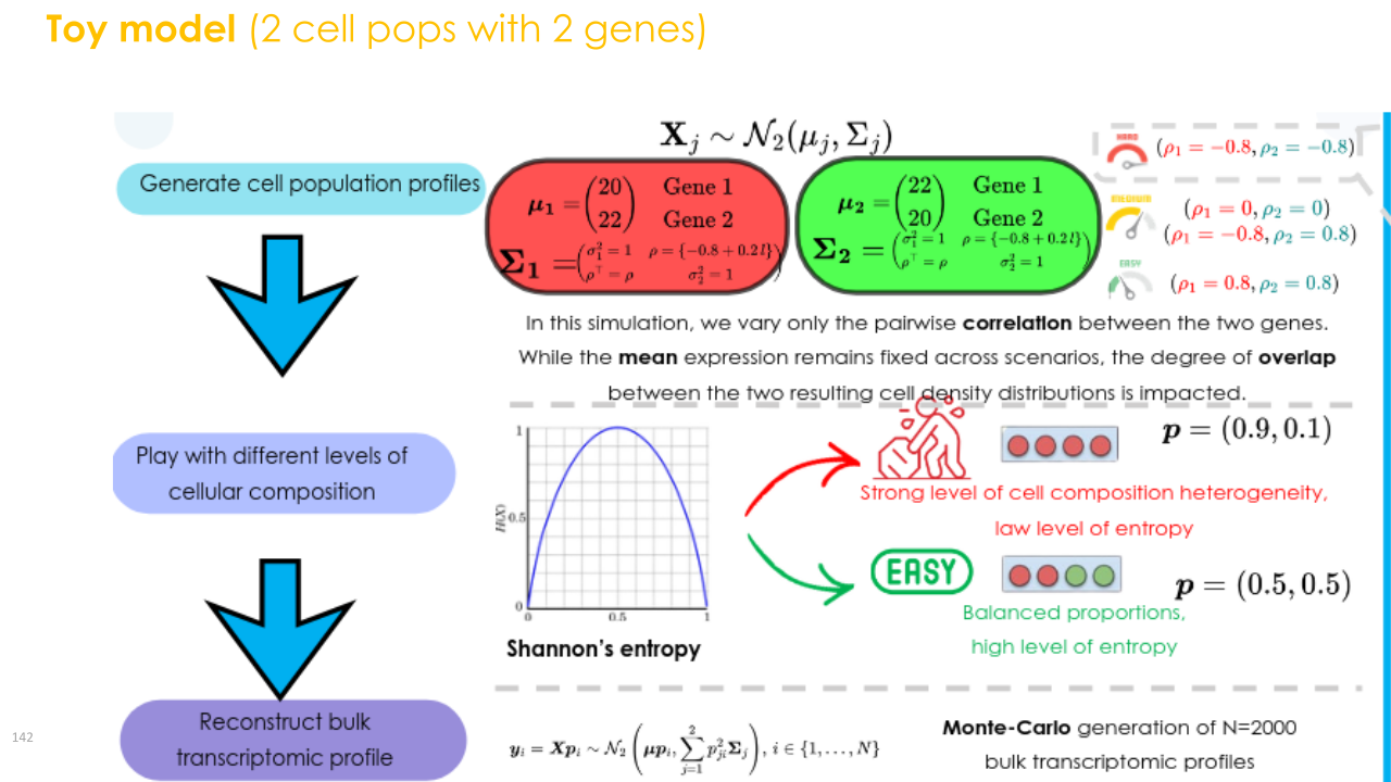
With p_1+p_2=1, only one free ILR coordinate is estimated (see derivatives under simplex transforms). Even when mean profiles are similar, gene–gene correlation can degrade mean-only solvers, and is partly recovered once \boldsymbol{\Sigma}(\boldsymbol{p})=\sum_j p_j^2\boldsymbol{\Sigma}_j enters the likelihood.
(a) Hyperparameter grid used in the bivariate manuscript study: two centroid geometries, balanced versus unbalanced \boldsymbol{p}, a gene–gene correlation sweep, and the first-generation plus DeCovarT solvers.
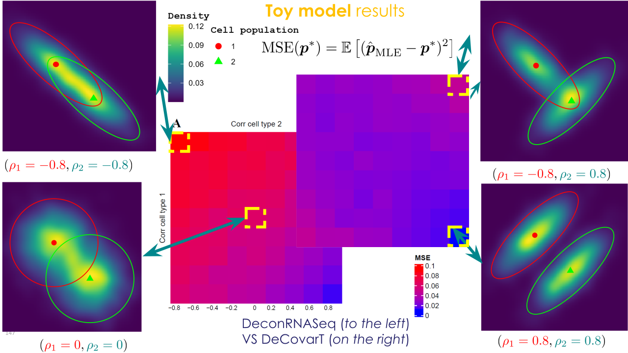
(b) AI-generated 2D density of the two-gene mixture while only the pairwise correlation changes, at fixed means, marginal variances, and composition. The ggplot panel below recomputes the same contrast and annotates MixSim overlap.
Figure 3: Factorial design (left) and correlation-only 2D densities (right) for the bivariate toy. {#fig-toy-design}
CLD is centroid (mean-profile) Euclidean separation \lVert\boldsymbol{\mu}_{\cdot 1}-\boldsymbol{\mu}_{\cdot 2}\rVert_2, not an Aitchison distance; see the descriptor notes. Small CLD uses \boldsymbol{\mu}_{\cdot 1}=(20,22), \boldsymbol{\mu}_{\cdot 2}=(22,20) (d=2\sqrt{2}\approx 2.83, cosine \approx 0.995). Large CLD uses (20,40) and (40,20) (d=20\sqrt{2}\approx 28.3, cosine 0.8).
Scenario ID
Each row is labelled B{index}_{variance}_{composition}_{CLD}. The index is the factorial row number (1–972). Example: B1_Ho_Ba_Sm is the first row, homoscedastic, balanced proportions, small CLD.
The slim design grid is output/fig02/bivariate_config.rds (no true_theta). Geometry, MixSim BarOmega, Hellinger, and Jeffreys live in bivariate_descriptors.rds. Convolution parameters are bivariate_theta.rds. ADEMP metrics (regression, monte_carlo, optimisation, call) are bivariate_benchmark.rds. All four files share the ID key. read_simulation_artefacts(dir, "bivariate", assemble = TRUE) rejoins them for plotting.
The Monte Carlo \hat{\boldsymbol{p}} draws themselves are the cell-type columns of optimisation (one row per replicate \times algorithm \times scenario). pivot_mc_estimates() stacks those columns into long form. Interior Wald intervals for convolution-likelihood solvers use vcov_ilr_delta() (expected Fisher information through the ILR chart), matching confint.decovart_fit(). Coverage, mean_model_se, and se_sd_ratio (mean model SE / empirical SD) are then finite. Mean-only solvers (NNLS, LSEI) leave those Wald columns missing: they do not maximise the convolution likelihood, so an ILR interval would not apply.
For J=2 the free coordinate is p_1\in(0,1). The listing below evaluates \ell_{\boldsymbol{y}\mid\boldsymbol{\zeta}}(p_1,1-p_1) on one bulk draw. It is not executed during R CMD build: Quarto’s Windows CLI starts a new R process that cannot see the temporary library (quarto-r#217). The same likelihood path is checked in tests/testthat/.
set.seed(20260828)rho<-0.6R<-matrix(c(1, rho, rho, 1), nrow =2)Sigma<-array(c(R, R), dim =c(2, 2, 2))dimnames(Sigma)<-list(rownames(mu_small),rownames(mu_small),colnames(mu_small))y_one<-DeCovarT::simulate_bulk_mixture(mu_small,Sigma, p =p_bal, n =1)$Y[, 1]p1_grid<-seq(0.02, 0.98, by =0.01)ll_grid<-vapply(p1_grid,function(p1){DeCovarT::loglik_multivariate(c(p1, 1-p1), y_one, mu_small, Sigma)},numeric(1))ll_df<-data.frame(p1 =p1_grid, loglik =ll_grid)ggplot2::ggplot(ll_df, ggplot2::aes(x =p1, y =loglik))+ggplot2::geom_line(colour ="#1B4F72", linewidth =0.8)+ggplot2::geom_vline( xintercept =0.5, linetype ="dashed", colour ="grey30")+ggplot2::labs( x ="p1 (p2 = 1 - p1)", y ="Log-likelihood")+ggplot2::theme_bw(base_size =11)
Performance is summarised using the ADEMP framework (Morris et al. 2019): bias, RMSE, coverage of ILR Wald intervals (Wilson intervals on the coverage rate), SE/SD, and optimiser failure rate. Mean-only baselines have no convolution Wald SE.
config on the in-memory benchmark still carries Shannon entropy of \boldsymbol{p} and MixSim overlap for tests. Saved artefacts split that information: optimisation stores per-sample \hat{\boldsymbol{p}}, elapsed time, and memory; regression and monte_carlo are the composition and ADEMP blocks from compute_benchmark_metrics().
Visualisations
Figures are written from the split RDS (no ADEMP refit). Density books go to output/fig02/density_visualisations/; RMSE / MAE / Aitchison tiles, raincloud, quantile-dot raincloud, forest, KKT raincloud, stacked convergence, whitened-ILR Q-Q / \chi^{2} Q-Q / KS lollipops, similarity, solver-dot, runtime, and memory books go to output/fig02/performance_visualisations/. Tile heatmaps (ggplot2::geom_tile()) show RMSE, MAE, and Aitchison distance on the (\rho_1,\rho_2) plane: one PDF per metric, one page per meta-scenario (CLD () variance () composition), seven solver panels. Scenario factors are relevelled (small then large CLD; homoscedastic then heteroscedastic; balanced, moderately unbalanced, highly unbalanced) when artefacts are read, and solvers follow nnls, lsei, SA, gradient, LBFGS, Newton-Raphson, Marquardt-Levenberg. Density and performance books share the four correlation corners (\rho_1,\rho_2)\in\{(0,0),(-0.8,-0.8),(0.8,0.8),(-0.8,0.8)\} (2\times 2\times 3=12 pages). Similarity heatmaps compute Pearson (r) of paired () within each corner, with Ward D2 clustering of (1-r) and Ward merge heights on the right dendrogram. Wald forests drop NNLS, LSEI, and SA; solid whiskers are (1.96) times the expected-Fisher Wald SE at the true composition, dashed whiskers use the empirical Monte Carlo SD, and coloured geom_label boxes (one per cell type, matching fig03) report RMSE and coverage. The native-space log-likelihood surface uses a log10 colour scale of the relative likelihood (L/L) so boundary peaks are visible. The matching rgl book uses the same log10 relative-likelihood z-axis. Rainclouds plot (p) with solver fill and stroke and a bottom legend. A companion dotsinterval.pdf book replaces the bounded [0,1] KDE slab with quantile dots. Runtime and memory rainclouds use one page per meta-scenario, the four correlation corners on the x-axis, and a log10 y-axis. Solver-dot pages use the same 9-by-9 ((_1,_2)) grid as the RMSE heatmaps: colour is mean RMSE and size is mean Aitchison distance, with horizontal y-axis labels. ggplot data tables are saved under output/fig02/ggplot_rds/.
Tip 1: Other one-sample log-likelihood slices (not drawn)
The current loglik_rgl.pdf holds the two mean profiles fixed and varies only \boldsymbol{p} (or the ALR coordinates of \boldsymbol{p}). White diamonds mark p^{\star} and red circles the numerical MLE; a 3D legend repeats those two markers. Expected log-likelihood surfaces \mathbb{E}_{\boldsymbol{y}\mid\boldsymbol{p}^{\star}}[\ell(\boldsymbol{p};\boldsymbol{y})] are drawn separately as loglik_expected_surface_p.pdf and loglik_expected_ilr_profile.pdf (not overlaid on the one-draw books). Useful alternatives, left as outlook:
Hold \boldsymbol{p}^{\star} fixed and vary one column of \boldsymbol{\mu} (a mean-shift slice) to show how centroid collision flattens \ell.
Hold \boldsymbol{p}^{\star} and \boldsymbol{\mu} fixed and vary one correlation \rho_j, so the surface is a covariance diagnostic rather than a mixing-weight diagnostic.
Overlay several independent bulk draws as translucent surfaces to display sampling variability of \ell(\boldsymbol{p};\boldsymbol{y}).
Likelihood geometry and solver behaviour
The factorial heatmaps remain the right design summary: large CLD and \rho_j=0 make the mean map injective, so every solver is accurate; small CLD plus aligned correlations flatten the mean residual and raise RMSE off the diagonal \rho_1=\rho_2. That saddle is a statement about identifiability of \boldsymbol{\mu}\boldsymbol{p}, not about which numerical method is used. The pack in output/fig02/mle_explanation/ (scenario descriptors, ILR profiles evaluated at \boldsymbol{y}=\boldsymbol{\mu}\boldsymbol{p}^{\star}, expected-Fisher Wald standard errors, and Newton versus Marquardt forests) is what separates three mechanisms that the heatmaps mix: the shape of \ell(\boldsymbol{p};\boldsymbol{y}), the surrogate each solver actually minimises, and the chart / stopping rule that walks that surrogate.
What is being optimised
Mean-only NNLS and DeconRNASeq (lsei in limSolve) minimise a convex quadratic (\boldsymbol{y}-\boldsymbol{\mu}\boldsymbol{p})^{\top}
(\boldsymbol{y}-\boldsymbol{\mu}\boldsymbol{p}) on the simplex (Dessole et al. 2023; Gong and Szustakowski 2013; Soetaert et al. 2026). For a convex objective a local minimiser is global (Boyd et al. 2004, ch. 4), so those fits are unique solutions of the least-squares problem. They are not maximisers of the convolution log-likelihood: \boldsymbol{\Sigma}(\boldsymbol{p}) never enters the quadratic. When \boldsymbol{\mu}_{\cdot 1} and \boldsymbol{\mu}_{\cdot 2} are close, that quadratic is a ridge along the simplex. A strictly feasible QP with bound constraints then has vertices as KKT candidates, which is why mean-only fits pile up at (1,0) and (0,1) whenever the residual is uninformative. Simulated annealing explores the same non-concave \ell as DeCovarT but without curvature, so it is a robustness check, not an MLE.
The convolution solvers maximise the Gaussian-convolution log-likelihood of the MLE properties article (that article is pkgdown-only; this vignette is the CRAN-shipped companion). None of them inherits Boyd’s global certificate, because that likelihood is not concave. They differ in coordinates and damping:
L-BFGS-B (stats::optim) runs limited-memory BFGS with box constraints 0\le p_j\le 1(Byrd et al. 1995; Zhu et al. 1997), then closes the simplex by p/\sum p. The equality \mathbf{1}^{\top}\boldsymbol{p}=1 is not a constraint of the line search, so \boldsymbol{\Sigma}(\boldsymbol{p}) can approach singularity mid-iteration; the implementation guards that with a finite penalty. Faces of the cube remain admissible, which is how a limited-memory quasi-Newton method sits on a simplex face after renormalisation.
Newton-Raphson (stats::nlminb) and Marquardt-Levenberg (marqLevAlg; (Philipps et al. 2023, 2021)) work in ILR coordinates, so the walk stays in the relative interior until a coordinate diverges. Newton uses the analytic Hessian. Marquardt adds a Levenberg damping term so that the working matrix stays positive definite (Marquardt 1963) even when the Hessian of \ell is indefinite, and stops on the relative-distance-to-maximum (RDM) criterion: the ratio of optimisation error to statistical error (Commenges et al. 2006). On a plateau, RDM is a feature — further progress along a flat ridge does not change inferential accuracy — and a bias: the iterate can halt nearer the barycentre than the true face.
The gradient solver is ILR BFGS without a Hessian, so it inherits the chart but not Newton’s local quadratic rate. Boyd’s Newton analysis (quadratic convergence in a neighbourhood of a strict local maximiser with positive-definite Hessian) applies to nlminb only when the realised \ell is locally strongly concave. The bivariate small-CLD profiles are not.
One bulk, N=1
Every Monte Carlo replicate here is a singleG=2 bulk. The MLE is therefore the N=1 estimator of the finite-sample section: biased at O(1), with Wald SEs that describe the Monte Carlo spread of that one-observation maximiser, not a sampling experiment with growing N. Pooling N i.i.d. columns with a shared \boldsymbol{p}^{\star} is what would make \hat{\boldsymbol{p}}_N consistent. The ILR profiles in the pack are evaluated at the conditional mean\boldsymbol{y}=\boldsymbol{\mu}\boldsymbol{p}^{\star}, which isolates the log-determinant remainder; the forests average over random \boldsymbol{Y}.
Reading the twelve meta-scenarios
Numbers below are from forest_newton_marquardt.csv, theoretical_wald_se.csv, and the range of ilr_loglik_profiles.csv (max minus min of \ell(\rho) on the plotting grid).
Large CLD, balanced, \rho_j=0 (B567). The mean map is well conditioned. The ILR profile spans about 101 nats and \mathrm{SE}_{\rho}=0.071. Newton and Marquardt agree to numerical noise: bias of p_1 about 0, RMSE 0.024, coverage 0.96, and the empirical SD matches the expected-Fisher SE (0.025). This is the textbook interior MLE: strongly concave locally, RDM and Newton stop at the same point.
Large CLD, balanced, \rho_j=-0.8 (B487). Equal negative correlation inflates variance along the anti-diagonal of gene space but does not destroy the mean contrast. Profile range 56, \mathrm{SE}_{\rho}=0.095, RMSE 0.033 for both second-order solvers. Covariance-aware curvature is still enough.
Small CLD, balanced (B1, B81). Means (20,22) versus (22,20) almost collinear. Profile range drops to 1.2–1.7 nats; \mathrm{SE}_{\rho} is 0.95 (both \rho=-0.8) or 0.71 (\rho=0). RMSE of p_1 is 0.19–0.23 and Wald coverage is conservative (0.98–1). Marquardt is slightly less variable than Newton here (RMSE 0.192 versus 0.234 on B1): damping and RDM cut walks along the ridge, which for a balanced truth is a small bias toward 1/2 that happens to reduce RMSE. Mean-only QPs see an even flatter residual and are the ones that snap to vertices.
Highly unbalanced, small CLD (B325, B405, p^{\star}=(0.99,0.01)). The ILR chart sends the rare type to \rho\to+\infty. Fisher curvature in \rho collapses: \mathrm{SE}_{\rho} is 24 (both \rho=-0.8) or 20 (\rho=0), while the profile range on a finite grid is only 2.4–4.1 nats — a plateau, not a peak. Newton bias for p_1 is -0.22 and -0.18; Marquardt bias is -0.40 and -0.38. Both shrink toward the barycentre, Marquardt more so, exactly as RDM predicts on a flat tail. Coverage stays near 0.92–0.94 because the Wald interval is already huge. This is the geometry behind chi-bar-square calibration on a face (boundary LRTs): the tangent cone is a half-line, Wilks does not apply, and a Wald SE in ILR is not a calibrated rare-type interval.
Highly unbalanced, large CLD (B811, B891). The profile in \rho is not flat in the raw log-likelihood (range 218–392), because a 1\% contamination still shifts a well-separated mean. The ILR SE remains large (3.3 and 2.5) because a small p_2 is a long way out on the chart. Newton follows that peak: bias -0.017 and -0.010, RMSE 0.035 and 0.026, coverage 0.97. Marquardt does not: bias -0.26 and -0.29, RMSE 0.35 and 0.37, coverage 0.47 and 0.40. The damping / RDM pair stops in ILR before |\rho| is large enough to represent p_2=0.01. A sharp peak in p can still look like a long walk in \rho; Marquardt’s statistical stopping rule then under-shoots a rare type even when the convolution likelihood is informative. That failure is an optimiser-chart interaction, not a lack of covariance signal.
Moderately unbalanced rows sit between these extremes: small-CLD RMSE 0.23–0.31 with Marquardt again more barycentric; large-CLD RMSE about 0.03–0.04 with the two second-order solvers aligned.
What the heatmaps still add
The 9\times 9(\rho_1,\rho_2) tiles, which are not in the twelve-row explanation pack, remain the place to see mean-only methods lose first as |\rho| grows at small CLD, and to see DeCovarT retain the diagonal saddle. The pack’s message is narrower and sharper: with N=1, a plateau in ILR makes every interior solver noisy; Marquardt’s RDM is the right stop on a balanced ridge and the wrong stop on a rare type; Newton with a full Hessian tracks p^{\star} once the means separate; convex QPs solve a different problem and are entitled only to that problem’s unique minimiser.
Boyd, Stephen, Stephen P. Boyd, and Lieven Vandenberghe. 2004. Convex Optimization. 1st edn. Cambridge University Press; Cambridge University Press. https://doi.org/10.1017/cbo9780511804441.
Byrd, Richard H., Peihuang Lu, Jorge Nocedal, and Ciyou Zhu. 1995. ‘A Limited Memory Algorithm for Bound Constrained Optimization’. SIAM Journal on Scientific Computing 16 (5): 1190–208. https://doi.org/10.1137/0916069.
Commenges, Daniel, Helene Jacqmin-Gadda, Cecile Proust, and Jeremie Guedj. 2006. A Newton-Like Algorithm for Likelihood Maximization: The Robust-Variance Scoring Algorithm. arXiv. https://doi.org/10.48550/arxiv.math/0610402.
Dessole, Monica, Marco Dell’Orto, and Fabio Marcuzzi. 2023. ‘The Lawson-Hanson Algorithm with Deviation Maximization: Finite Convergence and Sparse Recovery’. Numerical Linear Algebra with Applications 30 (5): e2490. https://doi.org/10.1002/nla.2490.
Gong, Ting, and Joseph D. Szustakowski. 2013. ‘DeconRNASeq: A Statistical Framework for Deconvolution of Heterogeneous Tissue Samples Based on mRNA-Seq Data’. Bioinformatics (Oxford, England) 29. https://doi.org/10.1093/bioinformatics/btt090.
Marquardt, Donald W. 1963. ‘An Algorithm for Least-Squares Estimation of Nonlinear Parameters’. Journal of the Society for Industrial and Applied Mathematics 11. https://doi.org/10.1137/0111030.
Morris, Tim P., Ian R. White, and Michael J. Crowther. 2019. ‘Using Simulation Studies to Evaluate Statistical Methods’. Statistics in Medicine 38 (11): 2074–102. https://doi.org/10.1002/sim.8086.
Philipps, Viviane, Boris P. Hejblum, Mélanie Prague, Daniel Commenges, and Cécile Proust-Lima. 2021. ‘Robust and Efficient Optimization Using a Marquardt-Levenberg Algorithm with R Package marqLevAlg’. The R Journal 13. https://doi.org/10.32614/rj-2021-089.
Philipps, Viviane, Cecile Proust-Lima, Melanie Prague, Boris Hejblum, Daniel Commenges, and Amadou Diakite. 2023. marqLevAlg: A Parallelized General-Purpose Optimization Based on Marquardt-Levenberg Algorithm.
Soetaert, Karline, Karel Van den Meersche, and Dick van Oevelen. 2026. limSolve: Solving Linear Inverse Models.
Zhu, Ciyou, Richard H. Byrd, Peihuang Lu, and Jorge Nocedal. 1997. ‘Algorithm 778: L-BFGS-B: Fortran Subroutines for Large-Scale Bound-Constrained Optimization’. ACM Transactions on Mathematical Software 23 (4): 550–60. https://doi.org/10.1145/279232.279236.