
2.2 Covariance-driven scenario (G = 20, J = 3)
Full script: scripts/fig03_variance_driven.R
2026-10-01
Source:vignettes/fig03-covariance-driven.qmd
The bivariate toy confirms the theoretical benefit of covariance modelling in a transparent setting but cannot demonstrate realistic gene-regulatory network (GRN) topology. This scenario uses G = 20 genes and J = 3 cell types in which types 1 and 2 are mean-collinear (\cos(\boldsymbol{\mu}_{\cdot 1},\boldsymbol{\mu}_{\cdot 2})=0.9): the network topology encoded in \boldsymbol{\Sigma}_j is the remaining discriminative signal. Construction, ADEMP benchmark, and the static network figure live in a single script, scripts/fig03_variance_driven.R (seed 20260807).
%%{init: {"theme": "sandstone"}}%%
flowchart TD
  P["3 compositions<br/>H* = 1 / 0.5 / 0.1"] --> S["36 scenarios"]
  G["2 x 2 graph assignments<br/>CT1, CT2: scale-free / cluster SBM"] --> S
  C["CT3 graph held at scale-free"] --> S
  K["3 target BarOmega levels<br/>low / moderate / high"] --> S
  S --> A["5 deconvolution solvers"]
%%{init: {"theme": "sandstone"}}%%
flowchart TD
P["3 compositions<br/>H* = 1 / 0.5 / 0.1"] --> S["36 scenarios"]
G["2 x 2 graph assignments<br/>CT1, CT2: scale-free / cluster SBM"] --> S
C["CT3 graph held at scale-free"] --> S
K["3 target BarOmega levels<br/>low / moderate / high"] --> S
S --> A["5 deconvolution solvers"]
---
config:
  layout: elk
  theme: sandstone
---
flowchart TB
  ROOT["Covariance-driven G=20, J=3"]
  ROOT --> SfSf["CT1 SF, CT2 SF"]
  ROOT --> SfSb["CT1 SF, CT2 SBM"]
  ROOT --> SbSf["CT1 SBM, CT2 SF"]
  ROOT --> SbSb["CT1 SBM, CT2 SBM"]
  SfSf --> SfSfLo["Low overlap"]
  SfSf --> SfSfMo["Moderate overlap"]
  SfSf --> SfSfHi["High overlap"]
  SfSb --> SfSbLo["Low overlap"]
  SfSb --> SfSbMo["Moderate overlap"]
  SfSb --> SfSbHi["High overlap"]
  SbSf --> SbSfLo["Low overlap"]
  SbSf --> SbSfMo["Moderate overlap"]
  SbSf --> SbSfHi["High overlap"]
  SbSb --> SbSbLo["Low overlap"]
  SbSb --> SbSbMo["Moderate overlap"]
  SbSb --> SbSbHi["High overlap"]
--- config: layout: elk theme: sandstone --- flowchart TB ROOT["Covariance-driven G=20, J=3"] ROOT --> SfSf["CT1 SF, CT2 SF"] ROOT --> SfSb["CT1 SF, CT2 SBM"] ROOT --> SbSf["CT1 SBM, CT2 SF"] ROOT --> SbSb["CT1 SBM, CT2 SBM"] SfSf --> SfSfLo["Low overlap"] SfSf --> SfSfMo["Moderate overlap"] SfSf --> SfSfHi["High overlap"] SfSb --> SfSbLo["Low overlap"] SfSb --> SfSbMo["Moderate overlap"] SfSb --> SfSbHi["High overlap"] SbSf --> SbSfLo["Low overlap"] SbSf --> SbSfMo["Moderate overlap"] SbSf --> SbSfHi["High overlap"] SbSb --> SbSbLo["Low overlap"] SbSb --> SbSbMo["Moderate overlap"] SbSb --> SbSbHi["High overlap"]
Generative model
One fixed mean signature \boldsymbol{\mu}\in\mathbb{R}^{G\times J} is built with generate_mean_signature_matrix() and an explicit Gram target_gram (mean signature construction). There is no marker block and no null (equal_all) block: uninformative genes would be removed before deconvolution.
R = \begin{pmatrix} 1 & 0.9 & 0.1 \\ 0.9 & 1 & 0.1 \\ 0.1 & 0.1 & 1 \end{pmatrix}, \qquad \boldsymbol{\mu} = s\mathbf{Q}R^{1/2}, \quad s=10. \tag{1}
Because \mathbf{Q}^{\mathsf{T}}\mathbf{Q}=\mathbf{I}_J, the pairwise cosines of the columns of \boldsymbol{\mu} equal R exactly (up to rounding). Euclidean gaps follow \lVert\boldsymbol{\mu}_{\cdot j}-\boldsymbol{\mu}_{\cdot k}\rVert
=s\sqrt{2(1-R_{jk})}. The call uses nonnegative = TRUE (disjoint gene-block frame) so that \boldsymbol{\mu}\ge 0, as required by deconvolute_ratios().
target_gram, mean_scale =10).
| pair | cosine | Euclidean |
|---|---|---|
| celltype_1 vs celltype_2 | 0.9 | 10\sqrt{0.2}\approx 4.472 |
| celltype_1 vs celltype_3 | 0.1 | 10\sqrt{1.8}\approx 13.416 |
| celltype_2 vs celltype_3 | 0.1 | 10\sqrt{1.8}\approx 13.416 |
Each of the mean-collinear types (CT1, CT2) independently draws an undirected skeleton from one of two generators, then completes a signed precision with build_normalised_precision() (GGM networks; topology families in the topology table):
-
Scale-free (
graph_model = "scale_free"): Barabási–Albert preferential attachment (power = 1,edges_per_node = 1). -
Cluster / stochastic block model (
graph_model = "stochastic_block_model"): three blocks with probabilities (0.5,0.25,0.25), p_{\mathrm{within}}=0.25, p_{\mathrm{between}}=0.01.
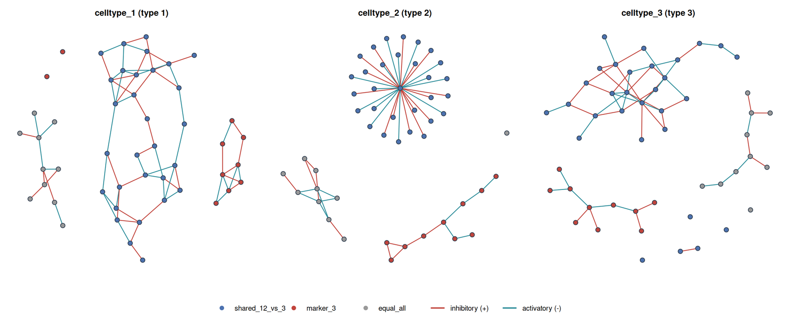
Erdős–Rényi is not used. Type 3, already separated by the Gram (R_{13}=R_{23}=0.1), is held at scale-free, so the topology factorial is 2^{2}=4 assignments on CT1 and CT2. Those generator names and parameter lists are stored on every row of hybrid_config.rds as graph_ct1 / graph_ct2 / graph_ct3 and the list-column graph_generators, and again inside each true_theta.
The spectral cushion u used at completion is now a fixed engineering constant (PRECISION_SHIFT_BASE = 0.2) so that each graph has one SPD precision. The experimental knob is a global covariance scale s: \boldsymbol{\Sigma}_j\mapsto s\boldsymbol{\Sigma}_j keeps every structural zero of \boldsymbol{\Omega}_j because \boldsymbol{\Omega}_j(s)=\boldsymbol{\Omega}_j/s. scale_covariances_to_overlap() searches s so that MixSim BarOmega matches a target in \{0.02,0.08,0.20\} (low / moderate / high), using Sobol Monte Carlo for G=20 (overlap note). This is the graph-constrained analogue of MixSim / FSDA average-overlap simulation (CRAN MixSim; (Melnykov et al. 2012; Riani et al. 2015)): we do not call MixSim() as a generator, because it cannot take a precision support as input.
Larger s also raises the covariance-information fraction f_{\mathrm{cov}} (mean Fisher scales as 1/s; the covariance block is scale-invariant). See the tangent-Fisher callout.
| Factor | Levels |
|---|---|
| Graph model (CT1, CT2) | scale-free; cluster SBM |
| Graph model (CT3) | scale-free (fixed) |
Target BarOmega
|
low (0.02); moderate (0.08); high (0.20) |
| Topology assignments | 2^{2}=\mathbf{4} |
| Covariance draws | 4\times 3=\mathbf{12} |
describe_simulation_scenario() records the realised BarOmega, f_{\mathrm{cov}}, \kappa\{\boldsymbol{\Sigma}(\boldsymbol{p})\}, and pairwise AIRM distance of the \boldsymbol{\Sigma}_j on every row. The overlap target is matched at the balanced composition; unbalanced \boldsymbol{p} change MixSim’s MAP weights, so realised BarOmega is higher there. AIRM is invariant to the global scale s (it scores topology / shape). f_{\mathrm{cov}} rises with s.
Two generators were considered but not adopted:
- Toeplitz covariances: encode only local (banded) dependencies; cannot model cell-type-specific sparse precision.
-
MixSim()as a mixture generator: draws unconstrained means and covariances for a target average overlap; no graph-constrained precision input. DeCovarT keeps the graphs and matchesBarOmegaby scaling \boldsymbol{\Sigma}_j instead.
Inference
Compositions are one-dominant vectors from composition_from_entropy() targeting normalised Shannon entropy H^{\star}\in\{1,0.5,0.1\} (balanced; moderately unbalanced; highly unbalanced). All DeCovarT solvers start at the barycentre (initial_p = "barycentre"). Other initialisation strategies are reserved for separate scenarios.
| Factor | Levels |
|---|---|
| Composition \boldsymbol{p} | H^{\star}=1; H^{\star}=0.5; H^{\star}=0.1 |
| Algorithms | DeconRNASeq (lsei), CIBERSORT, L-BFGS-B, Newton–Raphson, Marquardt–Levenberg |
| Total scenarios | 4\times 3\times 3=\mathbf{36} |
N = 50 Monte Carlo replicates per scenario.
| Algorithm | Function | Constraint |
|---|---|---|
QP (DeconRNASeq-style) |
deconvolute_ratios_deconrnaseq |
simplex equality / inequality |
| CIBERSORT-style \nu-SVR | deconvolute_ratios_cibersort |
non-negative then repair_simplex()
|
| L-BFGS-B | deconvolute_ratios_L_BFGS_B |
ILR \to open simplex |
| Newton–Raphson | deconvolute_ratios_Newton_Raphson |
ILR / nlminb
|
| Marquardt–Levenberg | deconvolute_ratios_Marquardt_Levenberg |
ILR \to open simplex |
Mean-only baselines (LSEI, CIBERSORT) ignore \boldsymbol{\Sigma}_j. The three DeCovarT maps use the same convolution likelihood. The shipped catalogue (robust linear model, GLS, BFGS, simulated annealing) is listed in deconvolute_ratios().
N_REPLICATES <- as.integer(Sys.getenv("N_REPLICATES", unset = "50"))
ALGORITHMS <- c(
  "lsei",
  "cibersort",
  "LBFGS",
  "Newton-Raphson",
  "Marquardt-Levenberg"
)
# Full pipeline: Rscript scripts/fig03_variance_driven.R
Visualisations
| Output | Description |
|---|---|
output/fig03/density_visualisations/mean_signature.pdf |
Unscaled () heatmap |
output/fig03/density_visualisations/latent_projections.pdf |
16-page 2D latent-space book (Thomson / MCFA / MclustDR) |
output/fig03/density_visualisations/loglik_rgl.pdf |
3D ALR relative likelihood (rgl, log10 L/\max L; white diamond p^{\star}, red MLE, 3D legend) |
output/fig03/density_visualisations/loglik_expected_surface_p.pdf |
Expected log-likelihood on the ALR plane |
output/fig03/density_visualisations/network_topologies.pdf |
Graph skeletons, one page per MixSim overlap |
output/fig03/performance_visualisations/heatmap_rmse.pdf |
RMSE tiles |
output/fig03/performance_visualisations/heatmap_aitchison.pdf |
Aitchison tiles |
output/fig03/performance_visualisations/raincloud.pdf |
Monte Carlo \hat{\boldsymbol{p}} rainclouds (legend at the bottom) |
output/fig03/performance_visualisations/dotsinterval.pdf |
Quantile-dot companion (no bounded KDE slab) |
output/fig03/performance_visualisations/forest.pdf |
ADEMP Wald forest |
output/fig03/performance_visualisations/kkt_raincloud.pdf |
Projected-score KKT residual rainclouds |
output/fig03/performance_visualisations/convergence_stacked.pdf |
Theoretical success / numerical / theoretical failure |
output/fig03/performance_visualisations/qq_normal.pdf |
Whitened ILR versus N(0,1) (TS band) |
output/fig03/performance_visualisations/qq_chi2.pdf |
Joint D^{2} versus \chi^{2}_{J-1} |
output/fig03/performance_visualisations/ks_normal.pdf |
KS lollipops versus N(0,1) (reject below 0.05) |
output/fig03/performance_visualisations/runtime.pdf |
Solver wall-clock (log10 seconds) |
output/fig03/performance_visualisations/memory.pdf |
Peak memory (log10 MiB) |
Redraw with FIG03_POSTPROCESS_ONLY=1 Rscript scripts/fig03_variance_driven.R (no ADEMP refit). ggplot data tables go under output/fig03/ggplot_rds/.
Two-dimensional projections of a Gaussian convolution
With (G=20) the purified Gaussians and the bulk convolution are no longer drawable in the gene plane. The 16-page book latent_projections.pdf therefore maps each selected scenario to a 2D latent display. Pages keep the lowest and highest MixSim overlap (low / high; the moderate arm is omitted) and the highest and lowest Shannon entropy of () (balanced versus highly unbalanced), crossed with the four CT1/CT2 graph assignments ((2=16)). Each page is a (3) of scatterplots with 95% Gaussian ellipses, cell-type colour, axis labels that report the share of variability on the first two coordinates, a transparent cowplot scree inset of the first ten scaled eigenvalues, and a six-line footnote for panels A–F. Square panels use a unit aspect ratio (not coord_equal), so unequal factor-score ranges no longer squash the shared-plane row.
The three routes below all return an ordered set of eigenvalues that summarise how much variability sits in the plotted plane. They are not interchangeable with the DeCovarT likelihood: the bulk profile is a convolution of Gaussians, not a Gaussian mixture.
Warning 1
A J-type bulk draw is Y\mid\boldsymbol{p}\sim\mathcal{N}\bigl(\boldsymbol{\mu}(\boldsymbol{p}),\boldsymbol{\Sigma}(\boldsymbol{p})\bigr) with \boldsymbol{\mu}(\boldsymbol{p})=\sum_j p_j\boldsymbol{\mu}_{\cdot j} and \boldsymbol{\Sigma}(\boldsymbol{p})=\sum_j p_j^2\boldsymbol{\Sigma}_j. Every observation is a weighted sum of all types (
simulate_bulk_mixture()). A finite mixture instead draws a latent label and then one component, f(\boldsymbol{y})=\sum_k\pi_k\,\phi(\boldsymbol{y};\boldsymbol{\mu}_k,\boldsymbol{\Sigma}_k), with mixing weights () (not (^2)).MclustDRand mixtures of factor analysers target that mixture. Their (_k) are not cell-type proportions, and their component densities are not the convolution law used for deconvolution.
Independent factor analyses per cell type
The top row fits a two-factor Gaussian factor model separately to purified draws from each type (stats::factanal(), Thomson / regression scores (Thomson 1938)). The orthogonal-factor model is \boldsymbol{x}=\boldsymbol{\mu}+\Lambda\boldsymbol{f}+\boldsymbol{\varepsilon} with \boldsymbol{f}\sim N(\boldsymbol{0},I) and diagonal uniquenesses \Psi, so \boldsymbol{\Sigma}=\Lambda\Lambda^\top+\Psi. Thomson scores are the posterior mean \hat{\boldsymbol{f}}_R=E[\boldsymbol{f}\mid\boldsymbol{x}]=\Lambda^\top\boldsymbol{\Sigma}^{-1}(\boldsymbol{x}-\boldsymbol{\mu}). That is the natural probabilistic answer to “where does this 20-gene profile sit in the plane?”. Bartlett scores (uniqueness- weighted GLS) remain a factanal(..., scores = "Bartlett") sensitivity check and are not plotted. Gene-wise marginal variances are comparable after the global MixSim scale, so uniquenesses are less heterogeneous than in a typical psychometric battery. Independent per-type fits do not share a loading matrix: the three planes are not superimposed.
fit <- stats::factanal(
  X,
  factors = 2,
  rotation = "none",
  scores = "regression"
)
scores <- as.data.frame(fit$scores)
ggplot2::ggplot(scores, ggplot2::aes(Factor1, Factor2)) +
  ggplot2::geom_point() +
  ggplot2::coord_equal() +
  ggplot2::theme_classic()
Shared MCFA plane (EMMIXmfa)
The bottom-left and bottom-centre panels use mixtures of common factor analysers (McLachlan and Peel 2000; Rathnayake et al. 2024): a shared loading matrix A with \boldsymbol{\mu}_i=A\boldsymbol{\xi}_i and \boldsymbol{\Sigma}_i=A\Omega_i A^\top+D, so that posterior factor means live in one q=2 plane. The eigenvalues of A\bar{\Omega}A^\top+D are the scree inset.
-
Convolution (panel D). Bulk columns come from
simulate_bulk_mixture()(covariance weights p_j^2). MCFA is fitted to those unlabelled bulk draws, then the latent purified slices () from the same simulation are scored into that shared plane and coloured by true type. - Unsupervised mixture (panel E). Each draw is from one component with probability p_j (not p_j^2). MCFA does not use the labels; colour is the generating type, so the plot shows how well the shared factors recover overlap.
Supervised MclustDR plane
The bottom-right panel takes the same labelled mixture draws and fits mclust::MclustDA(..., modelType = "EDDA") then mclust::MclustDR() (Fraley et al. 2026; Scrucca 2010, 2015). See the MclustDR reference. The kernel blends between-class mean separation with covariance differences (lambda = 1 emphasises separation). The generalised eigenvalues (evalues) are the scree inset: they are cluster-relevant variability, not ordinary PCA variance. This is the right 2D plot if class labels are known. On bulk convolution draws a one-component Gaussian is the truth, so Mclust would split a single ellipsoid; that misspecified fit is not shown.
Solver runtime and memory
runtime.pdf and memory.pdf use the same composition order as the other performance books (balanced, then moderately unbalanced, then highly unbalanced): one page per (). Each page facets the three MixSim overlap levels, puts CT1/CT2 topology on the x-axis (SF/SF, SF/SBM, SBM/SF, SBM/SBM), and maps solver to colour, fill, and grouping. The geometry is a vertical ggdist half-eye (raincloud) of the per-sample optimisation$elapsed_sec or memory_bytes (converted to MiB), with a left-side geom_rug() of the raw Monte Carlo draws and a log10 y-axis.
Likelihood geometry and solver behaviour
Cell types 1 and 2 share cosine 0.9, so the mean map \boldsymbol{\mu}\boldsymbol{p} is close to singular in the (p_1,p_2) plane: type 3 is the only well-separated mean. MixSim \bar\omega then sets how much of the remaining signal lives in \{\boldsymbol{\Sigma}_j\}. The pack in output/fig03/mle_explanation/ (descriptors, ILR slices of \ell at \boldsymbol{y}=\boldsymbol{\mu}\boldsymbol{p}^{\star}, expected-Fisher SEs, Newton/Marquardt forests on balanced compositions, and a quantile-sampled raincloud across all H^{\star}) is the numerical reading of that geometry. As in the bivariate toy, three layers must be kept apart: the convolution \ell, the surrogate each solver optimises, and the chart / KKT / stopping rule.
Surrogates versus the convolution
lsei (limSolve) is again a convex QP for \|\boldsymbol{y}-\boldsymbol{\mu}\boldsymbol{p}\|_2^2 on the simplex (Soetaert et al. 2026; Gong and Szustakowski 2013; Dessole et al. 2023; Boyd et al. 2004). With two nearly collinear signature columns the QP is under-determined in the (p_1,p_2) direction; the equality \sum p_j=1 plus bounds then put mass on a face. CIBERSORT replaces squares by a \nu-SVR hinge (Newman et al. 2015). The dual is a convex quadratic programme solved by sequential working-set methods (Fan et al. 2005). The wrapper does not constrain coefficients to the simplex during the fit: negatives are clipped to zero and the remainder is renormalised. Clipping is a Euclidean projection onto the positive orthant, not a constrained MLE, so a support vector that overshoots becomes a vertex of \Delta^{2}. Neither method sees p_j^2\boldsymbol{\Sigma}_j.
DeCovarT solvers maximise the Gaussian convolution. Newton-Raphson and Marquardt-Levenberg do so in ILR, with a full Hessian versus Marquardt damping plus RDM (Marquardt 1963; Commenges et al. 2006; Philipps et al. 2021, 2023). L-BFGS-B uses a limited-memory inverse Hessian with box constraints on p, then p/\sum p (Byrd et al. 1995; Zhu et al. 1997). The same caveats as in the bivariate interpretation apply: Boyd’s local-quadratic Newton rate needs a locally strongly concave \ell; RDM stops when further ILR steps are smaller than statistical error; box-constrained BFGS may sit on a face after renormalisation. All of this is still N=1 per bulk (finite-sample MLE).
Balanced compositions (forest + Fisher)
The Newton/Marquardt forest in the pack is restricted to H^{\star}=1 (p^{\star}=(1/3,1/3,1/3)). On that slice the two second-order solvers are interchangeable. At low overlap (V1, both graphs scale-free) RMSE for p_1 is 0.113, bias 0.012, empirical SD 0.113, coverage 0.99. At high overlap (V7) RMSE rises only to 0.124 and coverage stays 0.99. Median RMSE for p_1 across the four graph assignments is 0.122 (low \bar\omega), 0.134 (moderate), 0.147 (high); type 3, whose mean is not collinear, stays easier at low overlap (median RMSE 0.064) and catches up as overlap grows (0.130). Expected-Fisher ILR standard errors in theoretical_wald_se.csv tell the same story: \mathrm{SE}_{\rho_1} goes from 0.63 (V1) to 0.97 (V7), and the condition number of the ILR information drops from 6.8 to 1.7 — not because the problem becomes better posed, but because both eigenvalues shrink and the ellipsoid becomes a large, round disk. Graph assignment (scale-free versus cluster SBM) moves those SEs by a smaller amount than \bar\omega does. Topology is visible; average overlap is the dominant knob, matching the design claim, for balanced p^{\star} and for second-order convolution MLEs.
Boundary pile-up (raincloud, all H^{\star})
The sampled raincloud (raincloud_sampled.csv) includes moderately and highly unbalanced Shannon targets. Among non-missing point estimates, 76\% of CIBERSORT values lie at 0 or 1. At the scenario-wise median (sample_role = q50), type 3 is exactly zero in 35 of 36 scenarios (mean \hat p_3=0.0008). That is the clip-and-renormalise step, not a convolution mode on a face. lsei sits on a bound in 42\% of sampled cells overall and in 58\% of highly unbalanced cells; LBFGS in 26\% and 36\%; Marquardt in 10\% and 17\%; Newton in 4\% and 12\%. On balanced raincloud rows Newton and Marquardt never hit \{0,1\}; LSEI still does (21\%). Mean-only and SVR methods convert a collinear mean map into a hard boundary estimate; ILR convolution methods convert it into a soft interior mode, until p^{\star} itself is a rare-type vertex.
Median absolute error of the q_{50} p_1 fit across scenarios is 0.048 (Newton), 0.100 (lsei), 0.114 (LBFGS), 0.142 (Marquardt), 0.159 (CIBERSORT). The Marquardt figure is not a contradiction of the balanced forest: on the highly unbalanced scenario V3 (p^{\star}\approx(0.980,0.010,0.010)) the q_{50} estimates are 0.92 (Newton), 0.93 (lsei), 1.00 (CIBERSORT), 0.82 (LBFGS), and 0.78 (Marquardt). LSEI is closer to the vertex because the QP wants a vertex; Marquardt is pulled toward the barycentre because RDM refuses a long ILR walk, the same mechanism as B811 in the bivariate pack. Covariance information therefore helps only if the solver actually follows the convolution ridge to the rare-type coordinate. A mean-only vertex can beat a damped interior MLE on raw p_1 error when the truth is already a vertex; it will still report \hat p_3=0 and cannot support a chi-bar-square test that the type is absent (boundary inference).
Ridges in the ILR slices
ilr_loglik_profiles.csv slices \ell(\rho_1,\rho_2) at \boldsymbol{y}=\boldsymbol{\mu}\boldsymbol{p}^{\star}. High \bar\omega produces ridges along the type-1/type-2 contrast (the collinear mean direction): many (\rho_1,\rho_2) give almost the same convolution Gaussian. Newton follows the ridge until the Hessian in the remaining well-identified direction (type 3 versus \{1,2\}) stops it. Marquardt stops earlier when RDM sees no inferential gain. L-BFGS-B, stepping in p with only box bounds, can leave the simplex during the line search and land near a face after p/\sum p, which is the raincloud’s 26\% bound rate. None of these paths is the Godambe sandwich or a Firth penalty (Firth 1993); both remain outlook (perspectives). With N=1, the honest frequentist statement for a rare type is still the restricted LRT / parametric bootstrap of the MLE article, not a Wald ellipse from vcov_ilr_delta().
See also
- Bivariate toy: §2.1
- Moment generator: How to build synthetic scenarios
- Overlap and SPD distances: Distances, overlap, and covariance information
- Feature-selection on this design: Appendix S6
- Identifiability of collinear means: Appendix S1