DeCovarT perspectives

Bastien Chassagnol

2026-10-01

Scope

Outlook on extending DeCovarT beyond the closed-reference Gaussian convolution. Sec. 1 fixes the index set. Sec. 3 derives the mean and the three covariance layers from single-cell replicates, then compares regression and probabilistic engines. Later sections cover Scheffé-type mixture structure, alternative observation laws, MAP / BLUP purification of sample-level profiles, CSNet-style type-level networks given known \boldsymbol{p}, sample-level covariates, incomplete references, isoforms, RNA–cell uncoupling, weighted / generalised least squares, Firth penalisation for few bulk samples, lineage and archetypes, time-resolved composition, ensembles, spatial transcriptomics, and multi-omics. Compositional reparametrisation is implemented in additive_logistic() and documented numerically in the derivatives under simplex transforms vignette. The same catalogue is tracked in GitHub issue 5.

Notation

Indices and random objects below are fixed for the rest of this vignette, including the single-cell extension in Sec. 3. They match the plate diagram in the package README.

Symbol	Meaning
g=1,\ldots,G	Gene
j=1,\ldots,J	Cell type
i=1,\ldots,N	Bulk sample
r=1,\ldots,R	Independent biological replicate in the single-cell reference
c=1,\ldots,C_{jr}	Cell of type j in replicate r
\boldsymbol{y}_{\cdot i}\in\mathbb{R}^{G}	Bulk profile of sample i
\boldsymbol{p}_{\cdot i}\in\Delta^{J-1}	Cell-number fractions; p_{ji}\ge 0, \sum_j p_{ji}=1
\boldsymbol{q}_{\cdot i}	RNA-mass fractions (see Sec. 4.5)
\boldsymbol{\mu}_{\cdot j}\in\mathbb{R}^{G}	Cross-replicate mean expression of one cell of type j
\boldsymbol{X}_{jrc}	Expression of cell c
\boldsymbol{M}_{jr}	Replicate-specific population mean of type j
\boldsymbol{\Sigma}_{W,j}	Within-replicate cell-to-cell covariance
\boldsymbol{\Sigma}_{B,j}	Between-replicate covariance of \boldsymbol{M}_{jr}
\boldsymbol{\Sigma}_{\mathrm{obs},i}	Residual bulk noise: diagonal, possibly heteroscedastic, no gene–gene correlation
S_j	Mean transcriptome size (RNA content) of type j
\boldsymbol{\theta}_{\cdot j}	Relative abundance inside type j, \sum_g\theta_{gj}=1, so \boldsymbol{\mu}_{\cdot j}=S_j\boldsymbol{\theta}_{\cdot j}
a_i>0	Sample-wise scale (depth, tissue size). Shared by all genes
\boldsymbol{d}\in\mathbb{R}^{G}_{+}	Optional gene-wise platform scale. Not free inside one bulk fit
\boldsymbol{x}_{\cdot j,i}\in\mathbb{R}^{G}	Latent purified profile of type j in sample i
\boldsymbol{\Omega}_j=\boldsymbol{\Sigma}_j^{-1}	Sparse precision of the type-j Gaussian graphical model

The current DeCovarT convolution (Eq. 2) is the special case in which each reference is one random population profile with covariance \boldsymbol{\Sigma}_j=\boldsymbol{\Sigma}_{B,j}, the sample scale is absorbed into \boldsymbol{y}_{\cdot i}, and both \boldsymbol{\Sigma}_{W,j} and \boldsymbol{\Sigma}_{\mathrm{obs},i} are omitted. \boldsymbol{\rho}_i in the README diagram is the unconstrained coordinate with \boldsymbol{p}_{\cdot i}=\psi(\boldsymbol{\rho}_i) the soft-max.

Bulk transcriptomic deconvolution is one instance of a mixture inverse problem: a composite signal (tissue expression, a spectrum, a chromatogram) is observed, and we seek the proportions \boldsymbol{p} of underlying components. Because \boldsymbol{p} is compositional (parts of a whole), estimates must lie on the simplex \Delta^{J-1}=\{\boldsymbol{p}\in[0,1]^J:\sum_j p_j=1\}. (Chassagnol et al. 2023) model each reference profile as multivariate Gaussian and recover \boldsymbol{p} by constrained maximum likelihood; classical deconvolution tools such as CIBERSORT assume gene-wise independence instead (Newman et al. 2015).

Mixture design and first-order structure

Mixture experiments and compositional data

DeCovarT—and bulk deconvolution more generally—sits inside the wider class of mixture inverse problems in formulation science, spectroscopy, and designed experiments where component fractions are explicit regressors on the simplex. R offers only a handful of packages for designed mixture points (as opposed to random \boldsymbol{p} on \Delta^{J-1}):

• AlgDesign (Wheeler 2025) — lattice and simplex-centroid mixture designs via genMixture() / gen.mixture(), plus D-, A-, and I-optimal designs; the closest general substitute for classical mixture DOE.
• skpr (Morgan-Wall and Khoury 2025) — optimal mixture designs from a candidate set under \sum_j p_j=1; preferable when optimality criteria matter more than fixed simplex-centroid lattices.

A modular Scheffé-type benchmark would combine AlgDesign (or skpr) to propose \boldsymbol{p}, DeCovarT (or baselines) to invert the mixture, and compositional metrics from the simulation vignettes.

In designed mixture experiments (chemistry, food science, formulation), component proportions are explicit regressors with no free intercept because \sum_j p_j=1. A Scheffé cubic model for three components reads

y = \beta_1 p_1 + \beta_2 p_2 + \beta_3 p_3 + \beta_{12} p_1 p_2 + \beta_{13} p_1 p_3 + \beta_{23} p_2 p_3 + \beta_{123} p_1 p_2 p_3, \tag{1}

with every p_j\in[0,1] and \sum_j p_j=1 (Brown et al. 2015; Aitchison 1982). DeCovarT’s current release implements only the first-order part of Eq. 1 in a probabilistic setting: for cell type j, reference mean \boldsymbol{\mu}_j and covariance \boldsymbol{\Sigma}_j are given, and the bulk mixture satisfies

\boldsymbol{Y}\mid\boldsymbol{p} \sim \mathcal{N}\!\left( \sum_{j=1}^{J} p_j\,\boldsymbol{\mu}_j,\; \sum_{j=1}^{J} p_j^{2}\,\boldsymbol{\Sigma}_j \right). \tag{2}

Eq. 2 is the Gaussian-convolution likelihood optimised in deconvolute_ratios(); it extends mean-only linear deconvolution by propagating gene–gene covariance, not by adding Scheffé interaction monomials.

Interaction and synergy terms

Synergy or antagonism between components corresponds to second-order terms in Eq. 1: a positive \beta_{12} means the joint presence of components 1 and 2 raises the response above the additive prediction \beta_1 p_1+\beta_2 p_2. A natural generative extension would enrich the mean and, optionally, the covariance:

\mathbb{E}[\boldsymbol{Y}] = \sum_j p_j\,\boldsymbol{\mu}_j + \sum_{j<k} f(p_j,p_k)\,\boldsymbol{\mu}_{jk} + \cdots, \tag{3}

\boldsymbol{\Sigma}(\boldsymbol{p}) = \sum_j p_j^{2}\,\boldsymbol{\Sigma}_j + \sum_{j<k} g(p_j,p_k)\,\boldsymbol{\Sigma}_{jk} + \cdots, \tag{4}

with f,g often taken as p_j p_k. Allowing \operatorname{Cov}(\boldsymbol {X}_j,\boldsymbol{X}_k)\neq\boldsymbol{0} relaxes DeCovarT’s independence assumption between components and captures non-additive mixing. Such a model remains compatible with the same simplex constraint on \boldsymbol{p} and could still be fitted by constrained MLE, at the cost of many additional interaction parameters and careful guard against overfitting.

The present generative framework keeps a linear mean map \boldsymbol{y}=\boldsymbol{\mu}\boldsymbol{p}. When the regression of a compositional response on Euclidean predictors is itself nonlinear, flexible simplicial nonparametric models (Tsagris et al. 2023) and folded \alpha-distributions on the simplex (Tsagris and Stewart 2020) are a natural outlook; they are not used in the current convolution.

Lineage-aware hierarchical deconvolution

Flat deconvolution treats every cell type as a sibling on one simplex. Hierarchical methods instead estimate proportions at several granularities linked by a cell-type tree: broad compartments first, then closely related subtypes whose mean signatures are collinear at the leaf level.

We reuse the DeCovarT set-up from the article: gene g=1,\ldots,G; cell type or tree node j; sample i=1,\ldots,N (independence across i). Slices follow the usual dot notation (\boldsymbol{\mu}_{\cdot j}, \boldsymbol{y}_{\cdot i}).

• \boldsymbol{y}=(y_{gi})\in\mathbb{R}_{+}^{G\times N}: bulk expression; \boldsymbol{y}_{\cdot i}\in\mathbb{R}_{+}^{G} is sample i.
• \boldsymbol{\mu}=(\mu_{gj})\in\mathbb{R}^{G\times J}: mean signature; \boldsymbol{\mu}_{\cdot j}\in\mathbb{R}^{G} is the cross-sample mean profile of type j (as in MuSiC (Wang et al. 2019)).
• \boldsymbol{p}=(p_{ji})\in\,]0,1[^{J\times N}: unknown relative proportions; \boldsymbol{p}_{\cdot i}\in\,]0,1[^{J} is the composition of sample i.

\boldsymbol{y}_{\cdot i}=\boldsymbol{\mu}\,\boldsymbol{p}_{\cdot i}, \tag{5}

\sum_{j=1}^{J} p_{ji}=1, \qquad p_{ji}\ge 0 \qquad (i=1,\ldots,N). \tag{6}

p_{j,i}=\sum_{c\in\mathcal{C}(j)} p_{c,i} \qquad (i=1,\ldots,N). \tag{7}

At each tree level the bulk mixture satisfies Eq. 5 with each composition on the unit simplex (Eq. 6). For a parent node j with child set \mathcal{C}(j), coherent hierarchical estimates require Eq. 7.

Hard versus soft lineage constraints

Despite diverse implementations, hierarchical bulk mRNA deconvolution methods fall into two constraint regimes:

• Hard constraints — child lineage ratios are forced to sum exactly to the parent estimate (Eq. 7). MuSiC and SCDC (tree-guided mode) first fix a parent total \hat{p}_{j,i}, then fit children q_{c,i} on the within-parent simplex so that \hat{p}_{c,i}=q_{c,i}\,\hat{p}_{j,i} (Wang et al. 2019; Dong et al. 2021). HIDE applies the same equality by renormalising child estimates after each top-down split (Völkl et al. 2025); Rectangle propagates coarse cluster fractions as hard bounds on fine-grained estimates (Eder et al. 2026).
• Soft constraints — parent–child coherence is encouraged but not enforced exactly. HiDecon adds a squared mismatch penalty to the deconvolution loss (Huang, Cai, Lu, et al. 2024); Kassandra trains separate predictors at predefined hierarchy levels without an explicit parent–child equality (Zaitsev et al. 2022).

Hard splitting after fixing the parent (Eq. 8):

\hat{p}_{c,i}=q_{c,i}\,\hat{p}_{j,i}, \quad q_{c,i}\ge 0,\; \sum_{c\in\mathcal{C}(j)} q_{c,i}=1. \tag{8}

HIDE renormalisation (Eq. 9):

\hat{p}_{c,i}\leftarrow \hat{p}_{c,i}\, \frac{\hat{p}_{j,i}}{\sum_{c'\in\mathcal{C}(j)}\hat{p}_{c',i}}. \tag{9}

HiDecon soft penalty (Eq. 10):

\mathcal{L}_{\mathrm{tot}} = \mathcal{L}_{\mathrm{deconv}} + \lambda\sum_{j}\sum_{i=1}^{N} \Bigl( p_{j,i}-\sum_{c\in\mathcal{C}(j)} p_{c,i} \Bigr)^{2}. \tag{10}

Within each regime, methods further differ by whether they reuse a single reference signature at every granularity or reselect / reweight genes locally at each internal node (Figure 1).

%%{init: {"theme": "sandstone"}}%%
flowchart TD
  A["Lineage-aware bulk mRNA deconvolution"] --> B{"Parent–child linkage"}
  B -->|"Hard equality (Eq. parent–child)"| C["MuSiC, SCDC, HIDE, Rectangle"]
  B -->|"Soft / uncoupled levels"| D["HiDecon, Kassandra"]
  C --> E{"Genes at each node"}
  D --> F{"Genes at each node"}
  E -->|"Fixed reference matrix"| G["SCDC ensemble"]
  E -->|"Node-local reweighting"| H["MuSiC, HIDE, Rectangle"]
  F -->|"Shared matrix + penalty"| I["HiDecon"]
  F -->|"Level-specific signatures"| J["Kassandra"]

Figure 1: Taxonomy of lineage-aware bulk mRNA deconvolution: parent–child constraint (hard vs soft) and reference-gene strategy (fixed matrix vs node-local weights).

xCell 2.0 (Angel et al. 2025) uses Cell Ontology ancestry to build signatures and control spillover between related labels, but its outputs are enrichment scores rather than a compositional tree; it sits outside the hard/soft fraction taxonomy above.

Table 1: Lineage-aware bulk mRNA deconvolution: constraint regime, enforcing equation, and gene strategy (2019–2026 census).

method	constraint	lineage constraint	gene strategy
MuSiC	Hard	Fix \(\hat{p}_{j,i}\); \(\hat{p}_{c,i}=q_{c,i}\hat{p}_{j,i}\), \(\sum_c q_{c,i}=1\)	Node-local consistent genes
SCDC	Hard (tree-guided)	MuSiC step; \(\hat{p}_{c,i}=q_{c,i}\hat{p}_{j,i}\)	Full reference; optional node split
HIDE	Hard	Fit then renormalise: \(\hat{p}_{c,i}\leftarrow\hat{p}_{c,i}\hat{p}_{j,i}/\sum_{c'}\hat{p}_{c',i}\)	Parent-specific learned weights
Rectangle	Hard (multiscale)	Coarse \(\boldsymbol{p}^{(\mathrm{coarse})}\) bounds fine estimates	Clustered + direct signatures
HiDecon	Soft	\(\mathcal{L}_{\mathrm{tot}}=\mathcal{L}_{\mathrm{deconv}}+\lambda\sum_{j,i}(p_{j,i}-\sum_c p_{c,i})^2\)	Shared $\boldsymbol{\mu}$; joint penalised fit
Kassandra	Soft / uncoupled	Separate models; no parent–child equality	Level-specific trained signatures
xCell 2.0	None (scores)	Ontology spillover control only	Ontology-aware signature generation

Table 1 and Figure 1 summarise the landscape aligned with Eq. 5–Eq. 7. Hard methods (MuSiC, HIDE, Rectangle) are easier to audit node by node but inherit upstream bias; soft coupling (HiDecon) can stabilise rare subtypes when the tree is credible. Node-local gene reweighting (MuSiC, HIDE, Rectangle) targets collinear siblings; fixed or level-specific signatures (SCDC, Kassandra) trade flexibility for simpler reference construction.

A natural DeCovarT extension would combine Eq. 2 with either Eq. 8 or Eq. 10, node-local marker panels, and ALR optimisation when a curated lineage tree is supplied—benchmarked at broad, intermediate, and terminal resolutions against HiDecon, HIDE, tree-guided MuSiC, and Rectangle. Spatial HIDF applies the same tree idea to spots with an RCTD back-end (Zou et al. 2026); scDETECT uses a lineage prior for differential expression rather than for \boldsymbol{p} (Xu et al. 2025). Archetypes and cell states (type versus shared gene-expression programmes) are taken up in Sec. 6.1.

Single-cell moments and population alignment

The signature that enters Eq. 2 is a population profile: one mean vector and one covariance per cell type. Single-cell counts are not that object. This section states how to build the mean and how the covariance splits, then how to place the resulting profiles on the same scale as bulk sample i.

Figure 2: Within-sample cell noise, between-replicate biological covariance, and residual bulk noise.

Figure 3: MuSiC assumptions for library-size normalisation: same population, conserved cell-size ratios, conserved library-size ratios, and the stronger A3-prime hypothesis for absolute cell-type fractions.

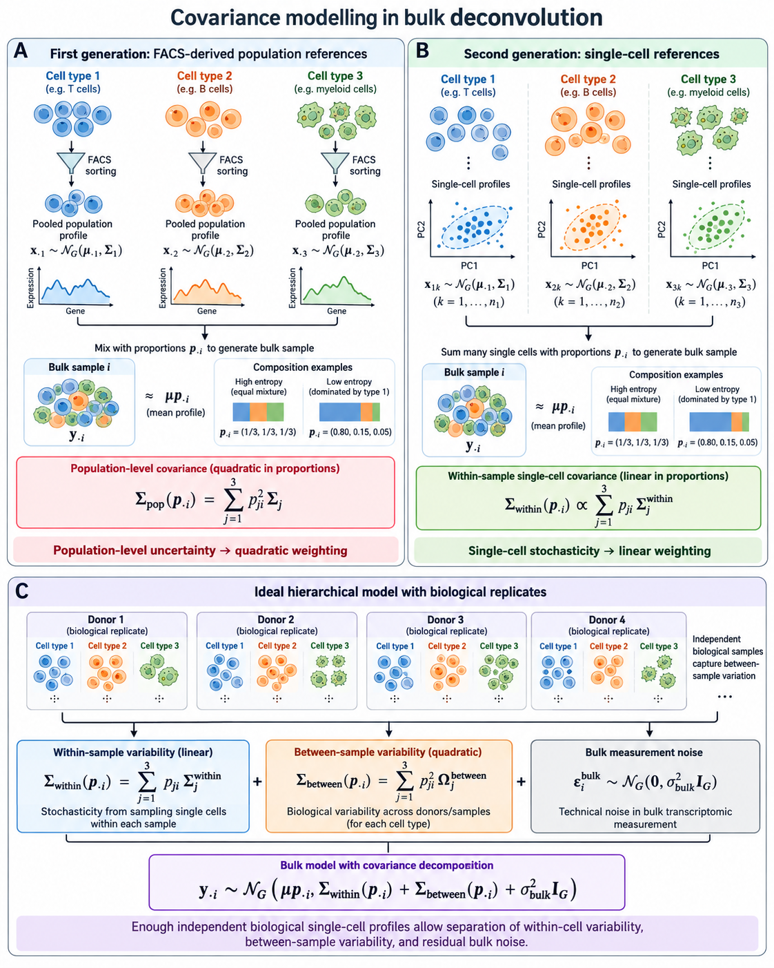
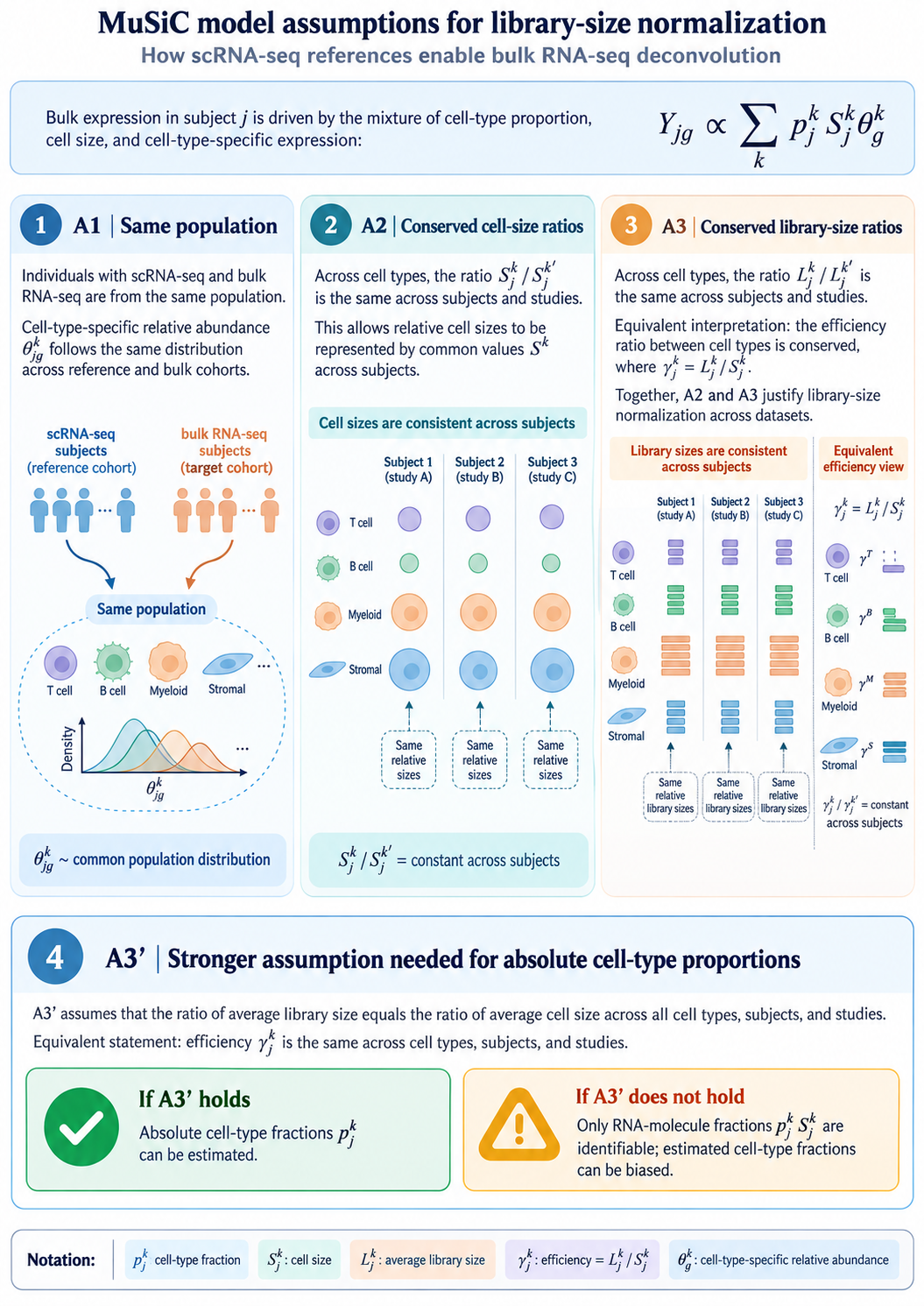
Figure 2 is the target decomposition. Panel A is a purified population profile (quadratic in p_{ji}). Panel B is one single-cell reference (linear in p_{ji}). Panel C is the hierarchical model once R independent replicates exist.

Mean: average cells, then average replicates

For a fixed type j, the per-cell mean does not depend on how many cells were captured. With raw counts on an additive scale,

\bar{\boldsymbol{X}}_{jr} = \frac{1}{C_{jr}}\sum_{c=1}^{C_{jr}}\boldsymbol{X}_{jrc}, \qquad \hat{\boldsymbol{\mu}}_{\cdot j} = \frac{1}{R}\sum_{r=1}^{R}\bar{\boldsymbol{X}}_{jr}. \tag{11}

Divide by the cell count C_{jr}, not by the library size. Library-size weights w_c=L_c/\sum_d L_d are functions of \boldsymbol{X}_c itself. Their probability limit is \boldsymbol{\mu}+\boldsymbol{\Sigma}\mathbf{1}/(\mathbf{1}^{\top}\boldsymbol{\mu}), so they target an RNA-weighted cell and destroy the exact Gaussian scale that leaves the precision graph unchanged. Under i.i.d. cells the arithmetic mean also has the largest effective sample size among deterministic convex weights.

Pool cells across replicates only after the within-replicate mean. A replicate with 10\,000 cells must not outweigh a replicate with 500 cells. MuSiC is built on that multi-subject split: cross-subject means and variances, with genes weighted by cross-subject and cross-cell consistency (Wang et al. 2019).

When every cell is scaled to a common total, the product S_j\boldsymbol{\theta}_{\cdot j} collapses to the arithmetic mean of the raw counts. MuSiC writes the signature as cell size times relative abundance and then recovers that same per-cell mean. Keep S_j and \boldsymbol{\theta}_{\cdot j} as separate factors (Sec. 3.3). Do not library-weight the raw vectors and call the result S_j.

Warning 1: Summing cells is the wrong signature, and the right pseudobulk

Summing is the correct total for a physical pool of exactly C_{jr} cells, \boldsymbol{T}_{jr}=\sum_c\boldsymbol{X}_{jrc}, with mean C_{jr}\boldsymbol{\mu}_{\cdot j} and covariance C_{jr}\boldsymbol{\Sigma}_{W,j}. Using \boldsymbol{T}_{jr} as a DeCovarT column inserts the arbitrary capture count into \boldsymbol{p}. A type with ten times more reference cells looks ten times more abundant.

The same sum is the right input for a different question. Differential expression of one cell type across donors needs one count vector per donor, then a bulk count model such as DESeq2 (Love et al. 2014). There the estimand is a relative fold change of averaged counts, and the donor is the independent unit. Cells from one donor are subsamples. Treating them as replicates inflates false discoveries (Squair et al. 2021). That analysis does not estimate \boldsymbol{p}_{\cdot i}.

Three reference regimes

Write the cell as a sum of a replicate effect and a cell effect,

\boldsymbol{X}_{jrc} = \boldsymbol{\mu}_{\cdot j}+\boldsymbol{B}_{jr}+\boldsymbol{\varepsilon}_{jrc}, \tag{12}

with \boldsymbol{B}_{jr}\sim\mathcal{N}(\boldsymbol{0},\boldsymbol{\Sigma}_{B,j}) and \boldsymbol{\varepsilon}_{jrc}\sim\mathcal{N}(\boldsymbol{0},\boldsymbol{\Sigma}_{W,j}), independent across j given \boldsymbol{p}_{\cdot i}. The bulk average per cell in a tissue of N_i cells is

\boldsymbol{A}_i = \sum_j p_{ji}(\boldsymbol{\mu}_{\cdot j}+\boldsymbol{B}_{jr(i)}) + \frac{1}{N_i}\sum_j\sum_{c=1}^{N_i p_{ji}}\boldsymbol{\varepsilon}_{ijc}. \tag{13}

FACS-sorted population profiles

Historically the reference was one bulk profile per purified population: surface-marker sorting, then a pooled microarray or RNA-seq library. The random object is the whole population vector \boldsymbol{Z}_{ij}\sim\mathcal{N}(\boldsymbol{\mu}_{\cdot j},\boldsymbol{\Sigma}_{B,j}), and the bulk is the convolution

\boldsymbol{y}_{\cdot i} = \sum_j p_{ji}\boldsymbol{Z}_{ij}, \qquad \operatorname{Cov}(\boldsymbol{y}_{\cdot i}\mid\boldsymbol{p}_{\cdot i}) = \sum_j p_{ji}^{2}\,\boldsymbol{\Sigma}_{B,j}. \tag{14}

The square appears because one random profile is multiplied by p_{ji}, not because p_{ji} cells were added. This is the covariance in Eq. 2. If several types are sorted from the same donors, cross-type blocks \boldsymbol{\Sigma}_{B,jk} add terms p_{ji}p_{ki}. Before droplet scRNA-seq, those population profiles came from FACS- or MACS-purified bulk libraries. Szaniszlo et al. showed that mixture expression reflects composition and that a minor subset is recovered only after physical sorting, while also stressing coexpression among genes inside a purified type (Szaniszlo et al. 2004). Novershtern et al. profiled 38 marker-defined haematopoietic populations and used coexpression modules plus promoter cis-circuits as the gene–gene structure of each state (Novershtern et al. 2011). Those studies are the historical FACS reference that Eq. 14 still describes.

One single-cell replicate (R=1)

R=1 identifies \boldsymbol{M}_{j1} and \boldsymbol{\Sigma}_{W,j}. It does not identify \boldsymbol{\Sigma}_{B,j}: extra cells shrink \boldsymbol{\Sigma}_{W,j}/C_{j1} and leave the single draw \boldsymbol{B}_{j1} untouched. The coherent bulk covariance is the mixture / physical sum, linear in p_{ji}:

\operatorname{Cov}(\boldsymbol{A}_i\mid\boldsymbol{p}_{\cdot i}) = \kappa_i\sum_j p_{ji}\,\boldsymbol{\Sigma}_{W,j} + \boldsymbol{\Sigma}_{\mathrm{obs},i}. \tag{15}

Here \kappa_i is an effective cells-per-bulk scale. The ideal value is 1/N_i. The number of reference cells C_{j1} is not N_i. A finite-cell reference mean adds a separate quadratic term \sum_j p_{ji}^{2}\boldsymbol{\Sigma}_{W,j}/C_{j1}. That term is Monte Carlo error of \hat{\boldsymbol{\mu}}_{\cdot j}, not biological between-donor covariance. Do not drop \boldsymbol{\Sigma}_{W,j} into the p_{ji}^{2} slot of Eq. 2.

For a rare type, p_{ji}=0.01 makes p_{ji}^{2} a hundred times smaller than p_{ji}. A within-cell covariance placed in the quadratic slot is almost silenced.

Enough biological replicates

The smallest R that identifies a variance component is R\ge 2. The replicate means satisfy

\bar{\boldsymbol{X}}_{jr} \sim \mathcal{N}\!\left( \boldsymbol{\mu}_{\cdot j},\; \boldsymbol{\Sigma}_{B,j}+\frac{\boldsymbol{\Sigma}_{W,j}}{C_{jr}} \right). \tag{16}

A method-of-moments contrast is then available. Let \boldsymbol{S}_{B,j} be the sample covariance of \{\bar{\boldsymbol{X}}_{jr}\}_{r=1}^{R} and \bar{C}_j a typical cell count. Then

\mathbb{E}[\boldsymbol{S}_{B,j}] = \boldsymbol{\Sigma}_{B,j} + \overline{\boldsymbol{\Sigma}_{W,j}/C_{jr}}, \tag{17}

so \hat{\boldsymbol{\Sigma}}_{B,j}=\boldsymbol{S}_{B,j}-\widehat{\boldsymbol{\Sigma}}_{W,j}/\bar{C}_j, projected onto the positive semidefinite cone. An unstructured G\times G covariance has G(G+1)/2 free entries. Transcriptome-scale G makes that matrix unestimable for the R of a normal single-cell study. What R\ge 2 buys is the scalar separation of the two layers, or a sparse precision for \boldsymbol{\Sigma}_{B,j}, not a dense G\times G matrix. Reference cohorts in current single-cell deconvolution are small; MEAD states this explicitly (Xie and Wang 2023). Cells from one donor share genetic and environmental background, so they are subsamples rather than independent biological units. Zimmerman, Espeland and Langefeld document that dependence across cell types, and they treat donor as the random effect when contrasting conditions (Zimmerman et al. 2021). That within-versus-between split is the same hierarchy as \boldsymbol{\Sigma}_{W,j} versus \boldsymbol{\Sigma}_{B,j} when a single-cell reference is aligned with bulk.

With that split, the bulk law DeCovarT should use is

\boldsymbol{y}_{\cdot i}\mid\boldsymbol{p}_{\cdot i} \sim \mathcal{N}\!\Big( a_i\sum_j p_{ji}\boldsymbol{\mu}_{\cdot j},\; \sum_j p_{ji}^{2}\,\boldsymbol{\Sigma}_{B,j} + \kappa_i\sum_j p_{ji}\,\boldsymbol{\Sigma}_{W,j} + \boldsymbol{\Sigma}_{\mathrm{obs},i} \Big). \tag{18}

\boldsymbol{\Sigma}_{\mathrm{obs},i} is diagonal. Gene–gene correlation is already inside \boldsymbol{\Sigma}_{B,j} and \boldsymbol{\Sigma}_{W,j}. Heteroscedastic diagonal entries are allowed. Off-diagonal residual correlation would double-count the network.

%%{init: {"theme": "sandstone", "flowchart": {"curve": "basis"}}}%%
flowchart TD
  ref["Reference used to build mu_j and Sigma_j"] --> facs["FACS-sorted population profiles"]
  ref --> r1["Single-cell reference, R = 1"]
  ref --> rR["Single-cell reference, R at least 2"]
  facs --> q["Quadratic convolution: sum p_ji squared Sigma_B,j"]
  r1 --> lin["Linear mixture: kappa_i sum p_ji Sigma_W,j"]
  rR --> both["Quadratic Sigma_B plus linear Sigma_W plus diagonal Sigma_obs"]
  lin --> noise["Plus diagonal residual Sigma_obs,i"]
  q --> noise

Figure 4: Which covariance terms are identified from the reference design. FACS profiles supply only the quadratic layer. One single-cell replicate supplies only the linear layer. R at least 2 separates both, plus a diagonal bulk residual.

Aligning reference profiles with bulk sample i

Eq. 11 is a per-cell mean. Bulk sample i is a library. Three scales sit between them. Only two belong inside the estimator.

Sample scale a_i. On an absolute molecule scale, \boldsymbol{y}_{\cdot i}=a_i\boldsymbol{\mu}\boldsymbol{p}_{\cdot i} plus noise. a_i absorbs cell number, sequencing depth, and capture. It is one positive number per bulk sample. Profile it out, or estimate it jointly with \boldsymbol{p}_{\cdot i}. It is not a biological composition parameter.

Cell size S_j. RNA content differs by cell type, so

\boldsymbol{y}_{\cdot i} = a_i\sum_j p_{ji} S_j\boldsymbol{\theta}_{\cdot j} + \boldsymbol{\varepsilon}_i. \tag{19}

MuSiC states the same product: cell fraction, average cell size, relative abundance (Wang et al. 2019). If S_j is measured, insert it. Do not re-estimate it. Free S_j and \boldsymbol{p}_{\cdot i} are not separately identifiable from \boldsymbol{y}_{\cdot i} alone, because only the products p_{ji}S_j enter Eq. 19. The RNA fraction

q_{ji} = \frac{p_{ji}S_j}{\sum_k p_{ki}S_k} \tag{20}

is what a normalised bulk identifies. \boldsymbol{q}_{\cdot i}=\boldsymbol{p}_{\cdot i} when S_j is constant across j. That constant-efficiency hypothesis is assumption A3' of MuSiC: the ratio of average library size equals the ratio of average cell size, equivalently a common capture efficiency \gamma_j=L_j/S_j (Figure 3). Under A3', the arithmetic mean across cells is the right signature and the fitted weights are cytometry fractions. If A3' fails, the fitted weights are RNA fractions and a later division by S_j (Eq. 34) is required.

EPIC and quanTIseq apply that division after a linear fit, using an external RNA-content assay, so the optimiser itself returns transcriptomic ratios (Racle et al. 2017; Finotello et al. 2019). MMAD estimates the extraction efficiencies inside a non-linear conjugate-gradient step (Liebner et al. 2014). ReDeconv keeps transcriptome size in the reference by Count-based Linearised Transcriptome Size (CLTS) normalisation, instead of dividing every cell by its own total (Lu et al. 2025).

Gene-wise scale \boldsymbol{d}. A platform shift can be gene-specific, y_{gi}\approx d_g a_i\sum_j p_{ji}\mu_{gj}. Bisque learns such a map from paired bulk and single-cell measurements when technical variation between the two assays is large (Jew et al. 2020). Fitting \{d_g\} on the same bulk sample that is being deconvolved lets the scale absorb any residual, and \boldsymbol{p}_{\cdot i} is then unidentified. Estimate \boldsymbol{d} on an external paired cohort, or do not estimate it.

Normalisation that preserves the linear mixture

The moment identities above are for raw counts on an additive scale. They do not survive a logarithm: \log\boldsymbol{y}_{\cdot i} is not \sum_j p_{ji}\log\boldsymbol{\mu}_{\cdot j}.

The comparison DeCovarT needs is the same gene on two technologies, not two genes inside one sample. Gene length is a property of the assay. It cancels for a within-gene contrast and should not be divided out of the reference unless the bulk was length-normalised in the same way. ReDeconv treats length as a bulk-only TPM/RPKM correction and leaves UMI single-cell counts uncorrected for length (Lu et al. 2025).

Procedure	What it estimates	Use for \boldsymbol{\mu}_{\cdot j}
Arithmetic mean of raw counts	Per-cell mean	Default signature
CPM / CP10K	Library-size relative profile	Erases S_j
TPM / RPKM / FPKM	Length-adjusted composition	Breaks cross-platform per-gene alignment
TMM (edgeR) or median-of-ratios (DESeq2)	Effective library size for differential expression	Donor-level DE, not the signature (Robinson et al. 2010; Love et al. 2014)
SCTransform	Regularised negative-binomial residuals	Clustering and integration, not an additive mixture mean (Hafemeister and Satija 2019)
CLTS (ReDeconv)	Counts rescaled by a linearised transcriptome size	Keeps S_j for deconvolution (Lu et al. 2025)

CPM and CP10K divide by the cell total. That is a relative profile \boldsymbol{\theta}_{\cdot j} with S_j discarded. TMM and the DESeq2 size factor answer a different question: an effective depth for between-sample differential expression, under a hypothesis that most genes are stable (Robinson et al. 2010; Love et al. 2014). SCTransform models depth inside a negative binomial; the residuals are not an additive convolution mean (Hafemeister and Satija 2019).

Tracks for a three-layer DeCovarT

Released DeCovarT is the FACS convolution: quadratic \boldsymbol{\Sigma}_{B,j}, no \boldsymbol{\Sigma}_{W,j}, no \boldsymbol{\Sigma}_{\mathrm{obs},i}. The extension in Eq. 18 adds the two missing layers and the scales a_i and S_j. Second-generation methods already implement pieces of that programme. The same symbols are used below. a_i is their sample scale, S_j their cell size, \boldsymbol{d} their gene-wise platform factor.

Regression engines

These methods treat \boldsymbol{\mu} as fixed once it has been averaged, and solve a simplex-constrained linear regression. They do not put a sampling law on \boldsymbol{y}_{\cdot i}.

%%{init: {"theme": "sandstone", "flowchart": {"curve": "basis"}}}%%
flowchart TD
  root["Regression: y_i = a_i mu p_i, p_i on the simplex"]
  root --> multi["Multi-subject reference"]
  root --> oneRef["One averaged signature"]
  multi --> music["MuSiC: weights by cross-subject and cross-cell consistency; keeps S_j"]
  multi --> music2["MuSiC2: same weights, iterative removal of condition-specific genes"]
  oneRef --> dwls["DWLS: dampened weighted least squares; average cells, sum to simulate bulk"]
  oneRef --> bisque["Bisque: gene-wise map d from paired bulk and single-cell"]
  oneRef --> tca["Wang 2022: matrix completion of the cell-type transcriptome"]

Figure 5: Regression-based single-cell deconvolution. All five methods share a linear mean and a simplex constraint. They split on how the reference is weighted and how the bulk is aligned.

Reference uncertainty. MuSiC down-weights genes whose cross-subject variance is large relative to their cross-cell variance, which is an empirical stand-in for \boldsymbol{\Sigma}_{B,j} versus \boldsymbol{\Sigma}_{W,j} (Wang et al. 2019). MuSiC2 keeps that weighting and iteratively removes genes that are differentially expressed between the reference condition and the bulk condition (Fan et al. 2022). DWLS averages cells to form \boldsymbol{\mu}_{\cdot j} and dampens high-leverage genes; the artificial bulk used for weighting is a sum of single-cell profiles, which matches Note 1. Bisque reduces single-cell noise by aggregating to a pseudobulk before learning \boldsymbol{d} (Jew et al. 2020). The 2022 matrix-completion preprint reconstructs the cell-type-resolution transcriptome rather than a single \boldsymbol{\mu}_{\cdot j}; it is a bulk completion method, not a covariance model (Wang et al. 2022). None of these five returns \boldsymbol{\Sigma}_{W,j} as a linear mixture weight. The same averaging of cells to a fixed \boldsymbol{\mu}_{\cdot j} is the first step of RCTD; the rest of that method is a Poisson–log-normal likelihood, treated in Sec. 3.4.2.

Alignment. MuSiC and MuSiC2 keep S_j inside the design and use a sample-level normalisation so that a_i does not have to be a free parameter (Wang et al. 2019; Fan et al. 2022). Bisque is the explicit \boldsymbol{d} method, estimated from the pairing of assays, not from the bulk sample alone (Jew et al. 2020). DWLS inherits whatever scale the averaged signature was built on (Tsoucas et al. 2019). CLTS is the normalisation that matches Eq. 19; CPM does not (Lu et al. 2025).

Generative model and estimation. The observation equation is ordinary or weighted least squares,

\hat{\boldsymbol{p}}_{\cdot i} = \arg\min_{\boldsymbol{p}\in\Delta^{J-1}} \|\boldsymbol{y}_{\cdot i}-a_i\boldsymbol{\mu}\boldsymbol{p}\|^{2}_{W}, \tag{21}

with W a diagonal gene-weight matrix. There is no likelihood, so there is no Fisher information for \boldsymbol{p}_{\cdot i}. Interval estimates, where they exist, come from resampling subjects (MuSiC) or from the regression sandwich, not from a Gaussian convolution. Assumptions shared by the family: additive scale, fixed library size after normalisation, \boldsymbol{\mu} independent of \boldsymbol{p}_{\cdot i}, and no residual gene–gene covariance inside the loss.

%%{init: {"theme": "sandstone", "flowchart": {"curve": "basis"}}}%%
flowchart TB
  subgraph plateR["r = 1 to R"]
    direction TB
    Xr["X_jr bar"]
  end
  mu["mu_j fixed"]
  Sj["S_j"]
  Xr --> mu
  subgraph plateI["i = 1 to N"]
    direction TB
    ai["a_i"]
    pi["p_i"]
    yi["y_i"]
    ai --> yi
    pi --> yi
  end
  mu --> yi
  Sj --> yi

Figure 6: Plate diagram for a regression engine. Reference replicates are collapsed to a fixed signature before the bulk plate is fitted.

Probabilistic engines, set against DeCovarT

RNA-Sieve and MEAD are errors-in-variables models: the design \boldsymbol{\mu} is observed with error, and a regression that ignores that error is attenuated (Erdmann-Pham et al. 2021; Xie and Wang 2023). DECALS keeps a subject-specific covariance but estimates \boldsymbol{p}_{\cdot i} by constrained least squares, with an asymptotic covariance that does not require a Gaussian bulk (Cai et al. 2024). ReDeconv, RCTD, and DeCovarT all put a parametric law on the bulk pointwise, not only in the large-gene limit. They differ in the law, in whether \boldsymbol{\mu}_{\cdot j} is random, and in the dependence on \boldsymbol{p}_{\cdot i}.

DECALS and MEAD are cited from the second-generation literature (Cai et al. 2024; Xie and Wang 2023), as are RNA-Sieve and ReDeconv (Erdmann-Pham et al. 2021; Lu et al. 2025). RCTD is written for spatial pixels; statistically it never uses neighbourhood structure, so each pixel is just an independent bulk sample i with library size N_i (Cable et al. 2022). Indices below follow Sec. 1 (gene g, type j, sample i), not the paper’s (j,k,i).

%%{init: {"theme": "sandstone", "flowchart": {"curve": "basis"}}}%%
flowchart TD
  root["Probabilistic deconvolution of y_i"]
  root --> eiv["Errors in variables: mu observed with error"]
  root --> cls["Constrained least squares, free of a bulk law"]
  root --> par["Parametric bulk law, pointwise"]
  eiv --> sieve["RNA-Sieve: gene-wise CLT, mean and variance"]
  eiv --> mead["MEAD: multivariate extension, gene-gene correlation, scales a_i and d"]
  cls --> decals["DECALS: subject-specific Sigma_i of p, constrained LS, asymptotic covariance"]
  par --> rctd["RCTD: Poisson-log-normal mixture of reads, mu fixed"]
  par --> rede["ReDeconv: univariate variances, linear in p, CLTS scale S_j"]
  par --> deco["DeCovarT: sparse multivariate Gaussian, quadratic in p"]

Figure 7: Probabilistic deconvolution split by how the bulk law depends on p. RNA-Sieve and MEAD share an errors-in-variables design. DECALS uses constrained least squares. RCTD is a read-level Poisson-log-normal mixture. ReDeconv and DeCovarT are parametric on averaged expression, univariate mixture versus sparse multivariate convolution.

Reference uncertainty. RNA-Sieve estimates a per-gene mean and variance from the reference cells and treats both the reference moments and the bulk as noisy. The marginal law of a random cell is a mixture; the bulk, as a sum of many cells, is handled by a central-limit normal likelihood. Dependence across genes is not a full \boldsymbol{\Sigma}_{W,j} (Erdmann-Pham et al. 2021). MEAD is the multivariate extension: the reference enters as a noisy design, gene–gene correlation is retained, and the model allows a sample scale and a gene-wise scale (Xie and Wang 2023). DECALS estimates cell-type-specific covariances from the bulk residuals themselves, because \operatorname{Cov}(\boldsymbol{y}_{\cdot i}) depends on \boldsymbol{p}_{\cdot i}, and then builds a subject-specific \boldsymbol{\Sigma}_i (Cai et al. 2024). It argues that the sandwich covariance used for MEAD does not consistently estimate that subject-specific matrix. ReDeconv uses a per-gene, per-type variance with linear weight p_{ji}, which is the diagonal of Eq. 15, together with CLTS so that S_j is not normalised away (Lu et al. 2025). RCTD averages library-normalised cells to a point \hat{\boldsymbol{\mu}}_{\cdot j} and then treats that vector as known (Cable et al. 2022). There is no \boldsymbol{\Sigma}_{B,j} and no \boldsymbol{\Sigma}_{W,j} in the bulk law: purified type expression is fixed, whereas DeCovarT treats it as a random population profile with known covariance. Residual gene-wise overdispersion \varepsilon_{gi} is the only randomness left around the mean. DeCovarT estimates a sparse precision per type and inserts it only as \boldsymbol{\Sigma}_{B,j}.

Alignment. RNA-Sieve rescales genes so that reference and bulk live on a comparable relative scale; the scale is not a free \boldsymbol{d} inside the simplex fit. MEAD writes \boldsymbol{y}_{\cdot i}=a_i\operatorname{diag}(\boldsymbol{d})\boldsymbol{X}_i\boldsymbol{p}_{\cdot i}+\boldsymbol{\varepsilon}_i and gives identifiability conditions under which \boldsymbol{p}_{\cdot i} survives an arbitrary \boldsymbol{d}. Those conditions are structural constraints on the signature, not “more bulk samples”. This matches the warning in Sec. 3.3. ReDeconv is the method that refuses CP10K precisely because it erases S_j (Lu et al. 2025). RCTD is the method that does estimate a gene-wise platform \boldsymbol{d}, but not from the sample being deconvolved. The reference mean is the arithmetic mean of \boldsymbol{X}_{jrc}/(\mathbf{1}^{\top}\boldsymbol{X}_{jrc}) over cells of type j, so S_j is already divided out (Sec. 3.3.1). On the bulk side, N_i is the observed library size (total UMIs) and acts as a GLM offset: it multiplies the mixture rate, exactly the proportional scaling a_i would play if depth were known. A remaining sample effect \alpha_i absorbs leftover capture. A gene-specific platform d_g is identified from a pseudobulk of all samples, because a free \boldsymbol{d} inside one fit would be interchangeable with \boldsymbol{p}_{\cdot i} (Sec. 3.3). After that plug-in, \hat{\boldsymbol{\mu}}_{\cdot j} is replaced by d_g\hat{\mu}_{gj}.

Generative model.

%%{init: {"theme": "sandstone", "flowchart": {"curve": "basis"}}}%%
flowchart TB
  subgraph plateR["r = 1 to R"]
    direction TB
    Bjr["B_jr"]
    Xbar["X_jr bar"]
    Bjr --> Xbar
  end
  mu["mu_j"]
  SB["Sigma_B,j"]
  SW["Sigma_W,j"]
  SB --> Bjr
  mu --> Xbar
  SW --> Xbar
  subgraph plateI["i = 1 to N"]
    direction TB
    ai["a_i"]
    pi["p_i"]
    eps["epsilon_i diagonal"]
    yi["y_i"]
    ai --> yi
    pi --> yi
    eps --> yi
  end
  mu --> yi
  SB -.->|"p_ji squared"| yi
  SW -.->|"kappa_i p_ji"| yi

Figure 8: Plate diagram for the three-layer extension of DeCovarT. Replicate plate r supplies Sigma_B and Sigma_W. Bulk plate i carries a_i, p_i, and a diagonal residual.

RCTD sits one layer below that plate. Each UMI is first assigned a type with probability p_{ji}, then a gene from that type’s relative profile: a read-level mixture, not a convolution of random population vectors (Cable et al. 2022). Conditional on the rate, the gene counts are Poisson; the rate is log-normal around a linear mixture of the fixed means. In DeCovarT symbols,

y_{gi}\mid\lambda_{gi} \sim \mathrm{Poisson}(N_i\lambda_{gi}), \qquad \log\lambda_{gi} = \alpha_i + \log\Bigl(\sum_j p_{ji}\mu_{gj}\Bigr) + \log d_g + \varepsilon_{gi}, \tag{22}

with \varepsilon_{gi} independent \mathcal{N}(0,\sigma_\varepsilon^2) (heavy-tailed in the implementation). The Poisson mean is therefore

\mathbb{E}[y_{gi}\mid\varepsilon_{gi}] = \underbrace{N_i e^{\alpha_i}}_{a_i} \, d_g \, e^{\varepsilon_{gi}} \sum_j p_{ji}\mu_{gj}. \tag{23}

N_i is observed depth; \alpha_i is a leftover sample scale; d_g is the gene-wise platform that DeCovarT’s \boldsymbol{d} names. The diagonal residual \varepsilon_{gi} is technical plus unmodelled gene-wise extra-Poisson noise, the count-scale cousin of \boldsymbol{\Sigma}_{\mathrm{obs},i}. Genes are independent given \varepsilon. Because \boldsymbol{\mu}_{\cdot j} is plugged in, Eq. 23 is a mixture of rates. DeCovarT’s Eq. 2 is a convolution of random type profiles: after averaging to a continuous expression vector, the bulk is \sum_j p_{ji}\boldsymbol{Z}_{ij} with \boldsymbol{Z}_{ij} Gaussian, hence quadratic in \boldsymbol{p}. A mixture is the right generative story at the UMI; a convolution is the right story at the aligned population mean.

%%{init: {"theme": "sandstone", "flowchart": {"curve": "basis"}}}%%
flowchart TB
  cells["library-normalised cells of type j"]
  mu["mu_j fixed"]
  d["d_g platform"]
  cells --> mu
  subgraph plateI["i = 1 to N"]
    direction TB
    Ni["N_i observed"]
    ai["alpha_i"]
    pi["p_i"]
    eps["epsilon_gi gene-wise"]
    yi["y_i Poisson"]
    Ni --> yi
    ai --> yi
    pi --> yi
    eps --> yi
  end
  mu --> yi
  d --> yi

Figure 9: Plate diagram for RCTD in DeCovarT notation. The reference is collapsed to a fixed mu_j. Sample i carries observed depth N_i, a leftover scale alpha_i, composition p_i, and a gene-wise overdispersion. Platform d is shared across samples and is not estimated inside the per-sample fit.

The fit is two-stage for the same identifiability reason as Sec. 3.3: \boldsymbol{d} cannot be free inside one sample.

%%{init: {"theme": "sandstone", "flowchart": {"curve": "basis"}}}%%
flowchart TD
  avg["Average library-normalised cells to mu_j"]
  filt["Keep differentially expressed genes"]
  pool["Pool samples to a pseudobulk S"]
  stage1["Stage 1: MLE of platform d and a bulk-wide mix W"]
  plug["Plug mu_j and d into the Poisson-log-normal"]
  stage2["Stage 2: per-sample SQP for w_ji = p_ji exp(alpha_i), w >= 0"]
  rec["Recover p_i by normalising w_i"]
  avg --> filt
  filt --> stage1
  pool --> stage1
  stage1 --> plug
  plug --> stage2
  stage2 --> rec

Figure 10: RCTD estimation. Stage 1 identifies the gene-wise platform from a pseudobulk. Stage 2 fits each sample independently by sequential quadratic programming on unnormalised weights w_ji = p_ji exp(alpha_i).

	Design error	Bulk law	Weight of type covariance	Scale	Estimator
RNA-Sieve	Yes, gene-wise	Asymptotic normal, genes separate	Variance, not a precision matrix	Relative rescaling	Maximum likelihood, asymptotic regions
MEAD	Yes, multivariate	Moment conditions, not a full density	Gene–gene correlation retained	a_i and \boldsymbol{d}, with identifiability conditions	Errors-in-variables estimator, delta-method intervals
DECALS	Through \boldsymbol{\Sigma}_i(\boldsymbol{p})	None	Subject-specific \boldsymbol{\Sigma}_i built from cell-type blocks	Absorbed before regression	Constrained least squares, asymptotic covariance
RCTD	No, \boldsymbol{\mu} plugged in	Poisson–log-normal mixture of reads, genes independent given \varepsilon	None	N_i known, \alpha_i and \boldsymbol{d}	Two-stage MLE; SQP on w\ge 0
ReDeconv	No	Univariate parametric, pointwise	Linear in p_{ji}	CLTS keeps S_j	Variance-aware regression
DeCovarT now	No	Sparse multivariate normal, pointwise convolution	Quadratic in p_{ji}	a_i profiled, S_j not in the likelihood	Constrained MLE on the ILR chart
DeCovarT in Eq. 18	Only via \boldsymbol{\Sigma}_{W,j}/C_{jr}	Same normal family	Quadratic \boldsymbol{\Sigma}_{B,j} plus linear \boldsymbol{\Sigma}_{W,j} plus diagonal \boldsymbol{\Sigma}_{\mathrm{obs},i}	a_i outside, S_j in the mean	Constrained maximum likelihood

RNA-Sieve and DeCovarT both obtain a normal bulk from a sum of random contributions. RNA-Sieve sums cells (linear variances, central limit, gene by gene). DeCovarT convolves population profiles (quadratic covariances, exact Gaussian, sparse precision). MEAD keeps the multivariate second-moment structure that RNA-Sieve drops, and adds the platform scales. DECALS wants the same subject-specific covariance but will not commit to a density; the price is a least-squares point estimate whose efficiency depends on how well \boldsymbol{\Sigma}_i is estimated. ReDeconv is the univariate, mixture-weighted cousin of the linear term in Eq. 18. RCTD is a read-level mixture with a Poisson–log-normal margin: each molecule comes from one type, \boldsymbol{\mu}_{\cdot j} is fixed, and extra-Poisson noise is gene-wise rather than a type-level \boldsymbol{\Sigma}_j.

SQP versus second-order descent. After stage 1, RCTD maximises a non-convex Poisson–log-normal log-likelihood in the unnormalised weights w_{ji}=p_{ji}e^{\alpha_i}, subject to w\ge 0 only (the simplex is recovered by normalising). The local quadratic Taylor model of that objective is a constrained quadratic programme. The Hessian is often indefinite, so a plain Newton step is not a descent direction; sequential quadratic programming keeps the positive-semidefinite part of the Hessian (eigenvalue clipping) and solves the QP with quadprog, a sequential convex programme in the sense of Duchi, reused from DWLS (Tsoucas et al. 2019). Inequality constraints and doublet/triplet cardinality penalties (active-set zeros) are native to that orthant formulation. DeCovarT instead maps \boldsymbol{p} to an unconstrained ILR chart and uses an analytic score and Hessian of a Gaussian convolution, with Marquardt damping when the Hessian is poorly conditioned. That second-order path is available because the observation is already an averaged, aligned intensity and the simplex is handled by the chart rather than by w\ge 0. It is the wrong local model for Eq. 22: the likelihood is non-convex in w, the support is the non-negative orthant, and many samples are expected to sit on a face.

The practical fork is the reference design, not a choice of optimiser.

• R=1. Fit Eq. 15. Report \boldsymbol{q}_{\cdot i} unless S_j is known, in which case apply Eq. 34 or insert S_j in Eq. 19. Do not publish \boldsymbol{\Sigma}_{W,j} as a DeCovarT \boldsymbol{\Sigma}_j. RCTD’s plugged-in \boldsymbol{\mu}_{\cdot j} is this regime’s mean; its Poisson–log-normal is an alternative observation law for the same R=1 design, not a substitute for \boldsymbol{\Sigma}_{B,j}.
• R\ge 2 with a sparse or low-rank between-replicate precision. Fit Eq. 18. The original quadratic term is then \boldsymbol{\Sigma}_{B,j} and has a sampling interpretation. \boldsymbol{\Sigma}_{\mathrm{obs},i} stays diagonal.

Statistical perspectives

The present estimator is a closed-reference, continuous, frequentist convolution: \boldsymbol{\mu}_{\cdot j} and \boldsymbol{\Sigma}_{j} are plug-in moments, and only \boldsymbol{p}_{\cdot i} is unknown. The subsections below change the observation law, the reference, or the loss, while keeping the simplex constraint (Eq. 6).

Alternative distributions

Split first by the support of \boldsymbol{y} (integer counts versus continuous intensities), then by frequentist plug-in versus Bayesian joint inference of \boldsymbol{p}_{\cdot i} and sample-level cell-type-specific (CTS) profiles \boldsymbol{x}_{\cdot j,i}.

%%{init: {"theme": "sandstone"}}%%
flowchart TD
  A["Bulk observation law"] --> B["Discrete counts"]
  A --> C["Continuous intensities"]
  B --> D["Multinomial / Dirichlet: ISOpureR, BayesPrism"]
  B --> LN["Multinomial logit-normal + gLasso"]
  B --> E["Poisson / PLN / ZIPLN: DeconV, Chiquet"]
  B --> RCTD["Poisson-log-normal mixture: RCTD"]
  C --> F["Univariate Gaussian: DSection, DeMix, BayICE"]
  C --> G["Multivariate Gaussian convolution: DeCovarT"]
  C --> RS["CLT Gaussian + noisy M: RNA-Sieve"]
  C --> H["Log-normal convolution: BLADE"]
  C --> CSN["Moments of the convolution: CSNet"]
  D --> I["Bayesian joint p and CTS"]
  G --> J["Frequentist plug-in mu, Sigma"]
  H --> I

Figure 11: Taxonomy of observation models for bulk deconvolution, relative to DeCovarT’s multivariate Gaussian convolution.

Measurement model versus expression model

Sarkar and Stephens review the count laws used for scRNA-seq by splitting every observation model into two pieces (Sarkar and Stephens 2021). The expression model is the law of the latent abundance. The measurement model is the conditional law of the observed counts given that abundance. Their default measurement model, for UMI data, is Poisson: the count for gene g in cell c is \mathrm{Poisson}(x_{c+}\lambda_{gc}), with x_{c+} the observed depth. A large fraction of zeros is then ordinary Poisson variation at a small rate. It is not a separate dropout event, and a zero is not a missing value: it still says that \lambda_{gc} is unlikely to be large.

What changes across methods is the expression model placed under that Poisson layer. A Gamma expression model yields a negative binomial observation. A point-Gamma expression model, a point mass at zero mixed with a Gamma, yields a zero-inflated negative binomial observation. Zero-inflation therefore belongs in the expression model when the data require it, and the review finds no support for a zero-inflated measurement model (including on spike-in controls). Multi-gene expression models add a low-rank factor for shared cell states on top of that gene-wise law. The discrete bulk laws below are the same split written for a mixture: multinomial and Poisson are measurement models; the Poisson–log-normal, ZIPLN and the logit-normal are expression models.

Discrete counts

A multinomial (or Dirichlet–multinomial) model treats \boldsymbol{y}_{\cdot i} as integer reads that sum to a library size. ISOpureR implements a hierarchical multinomial–Dirichlet purification of mixed tumour profiles (Anghel et al. 2015). BayesPrism places a multinomial likelihood on bulk counts with a patient-derived scRNA-seq prior and jointly infers \boldsymbol{p}_{\cdot i} and sample-level CTS expression (Chu et al. 2022). DeconV instead uses Poisson aggregation from single-cell to bulk (sums of independent Poissons remain Poisson) and returns interval estimates of \boldsymbol{p}_{\cdot i} (Gynter et al. 2023). RCTD is the Poisson–log-normal mixture of Eq. 22: each UMI picks a type, then a gene, with a gene-wise log-normal overdispersion and a two-stage platform correction (Cable et al. 2022); the comparison with DeCovarT’s convolution is in Sec. 3.4.2.

Over-dispersed, correlated counts are the domain of the multivariate Poisson–log-normal (PLN) family: a latent Gaussian vector induces dependence, and a Poisson observation layer yields integer reads (Chiquet et al. 2021, 2018). ZIPLN adds a Bernoulli zero-inflation layer for dropout (Batardière et al. 2025). A DeCovarT-style extension would replace Eq. 2 by a PLN (or ZIPLN) convolution on the latent log-abundance scale, keeping the ALR map on \boldsymbol{p}. A multinomial logit-normal on the gene simplex is a different discrete model: it is compositional association, not a cell-type convolution (Sec. 4.1.6).

Continuous intensities: frequentist versus Bayesian CTS

DeMixT (and DeMix) is the closest published convolution to DeCovarT: a frequentist Gaussian mixture of observed and latent components, but with independent genes and an unknown tumour or stromal profile (Wang et al. 2018; Ahn et al. 2013). DSection is a Bayesian univariate convolution (Normal / Gamma / Dirichlet priors and a Gibbs–Metropolis sampler) (Erkkilä et al. 2010). DeCovarT is frequentist, closed-reference, and multivariate: plug-in (\boldsymbol{\mu},\{\boldsymbol{\Sigma}_{j}\}), no unknown extra component, and a gene–gene residual network inside each \boldsymbol{\Sigma}_{j}.

RNA-Sieve is a supervised likelihood, but not that convolution (Erdmann-Pham et al. 2021). Their M, \alpha and b are DeCovarT’s \boldsymbol{\mu}, \boldsymbol{p} and \boldsymbol{y}. The bulk is modelled as the sum of n cells with a gene-wise central-limit Gaussian, plus measurement error in M (errors-in-variables). Genes are independent. Wald regions use the inverse Fisher information, or the Godambe sandwich under protocol shift. DeCovarT instead uses a full \boldsymbol{\Sigma}(\boldsymbol{p}) and plug-in moments; the resampling counterpart of noisy M is reference_bootstrap_decovart(). A side-by-side comparison is in the MLE properties vignette.

BLADE replaces the Gaussian with a gene-wise log-normal convolution, jointly purifying CTS profiles by variational inference (Andrade Barbosa et al. 2021). bMIND estimates sample-level CTS with an scRNA-seq-derived prior (Wang et al. 2020). The three Gaussian devices that recover \boldsymbol{x}_{\cdot j,i} given \boldsymbol{p}_{\cdot i} are in Sec. 4.1.4. The inverse problem that recovers type-level \boldsymbol{\mu}_{\cdot j} and a sparse second-moment network given \boldsymbol{p} is Sec. 4.1.5.

Zhang et al. benchmark joint \boldsymbol{p} + CTS engines and report BayesPrism with DWLS gene weights as the strongest combination on pseudobulk and real bulk data (Zhang et al. 2026). That is a weighted-likelihood analogue of Sec. 4.6.

MAP, BLUP, and the Wiener filter

Released DeCovarT estimates \boldsymbol{p}_{\cdot i} after plugging \boldsymbol{x}_{\cdot j,i} by \boldsymbol{\mu}_{\cdot j}. The latent profiles themselves remain recoverable once \boldsymbol{p}_{\cdot i} is treated as known. Write the convolution explicitly,

\boldsymbol{x}_{\cdot j,i} \sim \mathcal{N}(\boldsymbol{\mu}_{\cdot j},\boldsymbol{\Sigma}_j), \qquad \boldsymbol{y}_{\cdot i} = \sum_j p_{ji}\,\boldsymbol{x}_{\cdot j,i}, \tag{24}

independent across j given \boldsymbol{p}_{\cdot i}. Then \boldsymbol{y}_{\cdot i}\sim\mathcal{N}(\boldsymbol{\mu}\boldsymbol{p}_{\cdot i},\boldsymbol{\Sigma}(\boldsymbol{p}_{\cdot i})) with \boldsymbol{\Sigma}(\boldsymbol{p})=\sum_j p_{ji}^{2}\boldsymbol{\Sigma}_j as in Eq. 2. The joint law of (\boldsymbol{x}_{\cdot j,i},\boldsymbol{y}_{\cdot i}) is Gaussian, so three classical criteria coincide:

• the maximum a posteriori \arg\max_{\boldsymbol{x}_j} p(\boldsymbol{x}_j\mid\boldsymbol{y}_{\cdot i},\boldsymbol{p}_{\cdot i});
• the best linear unbiased predictor (Henderson) of the random effect \boldsymbol{x}_{\cdot j,i} in a linear mixed model whose variance components \boldsymbol{\mu}_{\cdot j} and \boldsymbol{\Sigma}_j are known;
• the Wiener filter, the linear minimum mean-square estimator of \boldsymbol{x}_{\cdot j,i} from \boldsymbol{y}_{\cdot i}.

All three equal the posterior mean

\hat{\boldsymbol{x}}_{\cdot j,i} = \boldsymbol{\mu}_{\cdot j} + p_{ji}\,\boldsymbol{\Sigma}_j\, \boldsymbol{\Sigma}(\boldsymbol{p}_{\cdot i})^{-1} (\boldsymbol{y}_{\cdot i}-\boldsymbol{\mu}\boldsymbol{p}_{\cdot i}). \tag{25}

If a diagonal residual \boldsymbol{\Sigma}_{\mathrm{obs},i} is present (Eq. 18), replace \boldsymbol{\Sigma}(\boldsymbol{p}_{\cdot i}) by \boldsymbol{\Sigma}(\boldsymbol{p}_{\cdot i})+\boldsymbol{\Sigma}_{\mathrm{obs},i}. The gain p_{ji}\boldsymbol{\Sigma}_j\boldsymbol{\Sigma}(\boldsymbol{p})^{-1} shrinks the bulk residual back onto type j in proportion to that type’s weight and covariance. The experimental helper scripts/experimental/03_04_DeCovarT_estimate_CTS_MAP_Bayesian.R is this update with \boldsymbol{\Sigma}(\boldsymbol{p}) assembled by .compute_global_variance(). A production path must pass the fitted \boldsymbol{p}_{\cdot i}, not a vector of ones.

bMIND is the same BLUP with an scRNA-seq prior on (\boldsymbol{\mu}_{\cdot j},\boldsymbol{\Sigma}_j) and a posterior mean per sample (Wang et al. 2020). BLADE replaces the Gaussian by a gene-wise log-normal and infers the latents variationally (Andrade Barbosa et al. 2021). Neither estimates a sparse \boldsymbol{\Omega}_j. Eq. 25 purifies one bulk column. It does not, by itself, re-estimate the type-level moments (\boldsymbol{\mu}_{\cdot j},\boldsymbol{\Sigma}_j) from a cohort.

Type-level moments given known proportions

CSNet inverts the DeCovarT arrow (Su et al. 2024). DeCovarT takes (\boldsymbol{\mu},\{\boldsymbol{\Sigma}_j\}) as plug-in and returns \boldsymbol{p}_{\cdot i}. CSNet takes \{\boldsymbol{p}_{\cdot i}\}_{i=1}^{N} as known (from CIBERSORT, MuSiC, or DeCovarT itself) and returns type-level means and a sparse correlation network. The generative identities are the same convolution as Eq. 24 and Eq. 2, written across a cohort rather than one sample:

\mathbb{E}[\boldsymbol{y}_{\cdot i}\mid\boldsymbol{p}_{\cdot i}] = \sum_j p_{ji}\,\boldsymbol{\mu}_{\cdot j}, \qquad \operatorname{Cov}(\boldsymbol{y}_{\cdot i}\mid\boldsymbol{p}_{\cdot i}) = \sum_j p_{ji}^{2}\,\boldsymbol{\Sigma}_j. \tag{26}

No Gaussian law is required for the moments. Let P\in\mathbb{R}^{N\times J} have entries P_{ij}=p_{ji} and H\in\mathbb{R}^{N\times J} have entries H_{ij}=p_{ji}^{2}. Gene-wise ordinary least squares on the linear mean recovers

\hat{\boldsymbol{\mu}}_{g\cdot} = (P^{\top}P)^{-1}P^{\top}\boldsymbol{y}_{g\cdot}, \tag{27}

the bulk analogue of a reference average, now identified from compositional contrast across samples rather than from purified cells. Centred residuals z_{gi}=y_{gi}-\sum_j p_{ji}\hat{\mu}_{gj} then satisfy the pairwise identity z_{gi}z_{g'i}=\sum_j p_{ji}^{2}\Sigma_{gg',j}+\varepsilon_{gg'i}. Least squares of the Hadamard products on H estimates each covariance entry,

\hat{\Sigma}_{gg',j} = \bigl[(H^{\top}H)^{-1}H^{\top}(\boldsymbol{z}_{g\cdot}\odot\boldsymbol{z}_{g'\cdot})\bigr]_{j}. \tag{28}

CSNet converts \hat{\boldsymbol{\Sigma}}_j to a correlation \hat{R}_j and applies an element-wise SCAD threshold. That is a marginal co-expression graph, not a Gaussian Markov precision. The Gaussian convolution log-likelihood in \{\boldsymbol{\Sigma}_j\}, which is the natural DeCovarT loss for the same parameters, is neither convex nor biconvex in those matrices; pairwise least squares is how CSNet avoids that optimisation (Su et al. 2024).

A DeCovarT-native sequel would keep Eq. 27–Eq. 28 as the moment step, then map \hat{\boldsymbol{\Sigma}}_j to a sparse precision \boldsymbol{\Omega}_j (graphical lasso, or SCAD on the inverse) so that the purified network is the same object DeCovarT already inserts into Eq. 2. That pipeline is in silico GRN inference run after \boldsymbol{p} has been estimated, not in place of it.

%%{init: {"theme": "sandstone", "flowchart": {"curve": "basis"}}}%%
flowchart TD
  bulk["Bulk matrix y over i = 1 to N"]
  plug["Plug-in mu_j and Sigma_j from a reference"]
  deco["DeCovarT: p_i given mu and Sigma"]
  map["MAP / BLUP / Wiener: x_j,i given y_i and p_i"]
  csnet["CSNet: mu_j and sparse R_j given y and p"]
  omega["Optional: sparse Omega_j from Sigma_j"]
  bulk --> deco
  plug --> deco
  deco --> map
  bulk --> map
  deco --> csnet
  bulk --> csnet
  csnet --> omega
  omega -->|"updated plug-in"| deco

Figure 12: Two inverse problems on the same convolution. DeCovarT estimates p given mu and Sigma. Given p, the MAP / BLUP recovers sample-level purified profiles, and CSNet recovers type-level means and a sparse co-expression network. A precision Omega_j estimated there can be fed back as the DeCovarT plug-in.

P and H must have full column rank, so \boldsymbol{p}_{\cdot i} has to vary across the N bulks. One sample identifies \boldsymbol{p} given (\boldsymbol{\mu},\{\boldsymbol{\Sigma}_j\}); it does not identify J covariance matrices. Rare types with almost constant p_{ji} leave the corresponding column of H weak, which is why CSNet recovers abundant-type co-expression more easily than microglia-scale weights. The method is a moment estimator: modest errors in the supplied \boldsymbol{p} are averaged over N, whereas DeCovarT’s likelihood for a single column is concentrated in \boldsymbol{p}_{\cdot i}.

	DeCovarT	MAP / BLUP (Eq. 25)	CSNet
Known	\boldsymbol{\mu}_{\cdot j}, \boldsymbol{\Sigma}_j (reference)	\boldsymbol{\mu}_{\cdot j}, \boldsymbol{\Sigma}_j, \boldsymbol{p}_{\cdot i}	\boldsymbol{p}_{\cdot i} (external or DeCovarT)
Unknown	\boldsymbol{p}_{\cdot i}	\boldsymbol{x}_{\cdot j,i} (one sample)	\boldsymbol{\mu}_{\cdot j}, sparse R_j (cohort)
Law	Multivariate Gaussian convolution	Same, posterior of the latents	Moments only; Gaussian optional
Second moment	Sparse precision \boldsymbol{\Omega}_j as input	Uses \boldsymbol{\Sigma}_j, does not re-estimate it	Sparse correlation R_j as output
Replication	One bulk column is enough	One bulk column	N\gg J bulks with varying \boldsymbol{p}
Estimator	Constrained MLE on the ILR chart	Posterior mean / Wiener gain	Gene-wise OLS, then pairwise LS, then SCAD

The two problems compose. Fit DeCovarT to obtain \hat{\boldsymbol{p}}_{\cdot i}; run Eq. 25 if the scientific target is a purified profile in that sample; run Eq. 27–Eq. 28 if the target is a type-level network; optionally replace the reference \boldsymbol{\Omega}_j by that network and refit \boldsymbol{p}. Do not treat a CSNet correlation graph as a DeCovarT precision.

Two simplices without convolution

McGregor et al. model a count vector of D features as compositional, not as a mixture of cell-type Gaussians (McGregor et al. 2026). In DeCovarT notation the features are the G genes. Sample i has library size n_i and gene composition \boldsymbol{\pi}_i\in\Delta^{G-1}. The observation is multinomial,

\boldsymbol{y}_{\cdot i}\mid n_i,\boldsymbol{\pi}_i \sim\mathrm{Multinomial}(n_i,\boldsymbol{\pi}_i), \qquad n_i\sim\mathrm{LogNormal}(\mu_n,\sigma_n^2), \tag{29}

with n_i\perp\boldsymbol{\pi}_i (read depth is treated as a technical scale). The composition is logit-normal on the ALR chart that uses gene G as the reference,

\boldsymbol{w}_i =\mathrm{alr}(\boldsymbol{\pi}_i) =\log(\pi_{1,i}/\pi_{G,i},\ldots,\pi_{G-1,i}/\pi_{G,i}), \qquad \boldsymbol{w}_i\sim\mathcal{N}_{G-1}(\boldsymbol{\mu}_w,\boldsymbol{\Sigma}_w), \qquad \boldsymbol{\pi}_i=\psi(\boldsymbol{w}_i), \tag{30}

where \psi is the additive logistic map already used for cell-type ratios (additive_logistic()). When G is large relative to the number of bulk samples, McGregor et al. penalise the Gaussian log-likelihood of the \boldsymbol{w}_i with a graphical lasso on the ALR precision \boldsymbol{\Omega}_w=\boldsymbol{\Sigma}_w^{-1} (Friedman et al. 2008), or the same \ell_1 penalty on the CLR precision (\mathbf{G}^{\mathsf{T}}\boldsymbol{\Sigma}_w\mathbf{G})^{-1}. That shrinks spurious gene–gene partial correlations. Their target is proportionality (\phi, \rho, log-ratio variances) on the latent \boldsymbol{\pi}_i, because empirical log-ratios of raw counts are biased by variation in n_i.

This is not DeCovarT’s convolution (Eq. 2). There is no mixing \sum_j p_j\boldsymbol{\mu}_j of purified profiles, and no \boldsymbol{\Sigma}(\boldsymbol{p})=\sum_j p_j^2\boldsymbol{\Sigma}_j. Current DeCovarT treats \boldsymbol{y}_{\cdot i} as an unbounded continuous intensity. Library size is omitted: the counts are not constrained to sum to n_i.

A fully compositional deconvolution would keep two simplices. Cell ratios \boldsymbol{p}_i\in\Delta^{J-1} stay on the existing ALR chart \boldsymbol{\rho}_i=\mathrm{alr}(\boldsymbol{p}_i). Gene composition stays on Eq. 30. The two can be coupled by a regression of the gene-ALR mean on \boldsymbol{p}_i, for example \boldsymbol{\mu}_w(\boldsymbol{p}_i)=\mathbf{B}\boldsymbol{p}_i, still without forming a Gaussian convolution of cell-type covariances. Figure 13 is that joint directed graph: grey circles are observed, white circles are latent, squares are parameters.

---
config:
  theme: sandstone
---
flowchart TB
  n(("$$n_i$$"))
  y(("$$\boldsymbol{y}_{\cdot i}$$"))
  pi(("$$\boldsymbol{\pi}_i$$"))
  w(("$$\boldsymbol{w}_i$$"))
  p(("$$\boldsymbol{p}_i$$"))
  rho(("$$\boldsymbol{\rho}_i$$"))
  mun["$$\mu_n,\sigma_n^2$$"]
  muw["$$\boldsymbol{\mu}_w(\boldsymbol{p}_i)$$"]
  Omegaw["$$\boldsymbol{\Omega}_w$$"]
  mur["$$\boldsymbol{\mu}_{\rho}$$"]
  Omegar["$$\boldsymbol{\Omega}_{\rho}$$"]

  mun --> n
  mur --> rho
  Omegar --> rho
  rho --> p
  p -.-> muw
  Omegaw --> w
  muw --> w
  w --> pi
  n --> y
  pi --> y

  classDef observed fill:#c8c8c8,stroke:#333,color:#111
  classDef latent fill:#ffffff,stroke:#333,color:#111
  classDef param fill:#f4f1ea,stroke:#333,color:#111
  class n,y observed
  class pi,w,p,rho latent
  class mun,muw,Omegaw,mur,Omegar param

Figure 13: Directed graph for a logit-normal multinomial gene composition (McGregor et al.) extended with a second simplex for cell-type ratios. Grey circles are observed. White circles are latent. Squares are parameters. The dashed arrow from p_i into mu_w is the optional deconvolution link; it is not a Gaussian convolution of Sigma_j.

Sample-level covariates

A condition, tissue, batch, sex or age vector \boldsymbol{z}_{i} is indexed by sample i, whereas \boldsymbol{\mu} has genes in rows and cell types in columns. Covariates therefore cannot be appended as extra columns of the signature. Two generative extensions are distinct (Fan et al. 2022).

State model. Condition alters the reference distribution,

\boldsymbol{x}_{\cdot j,i}\mid\boldsymbol{z}_{i} \sim\mathcal{N}_G \bigl(\boldsymbol{\mu}_{j}(\boldsymbol{z}_{i}),\boldsymbol{\Sigma}_{j}(\boldsymbol{z}_{i})\bigr), \tag{31}

for example \boldsymbol{\mu}_{j}(\boldsymbol{z}_{i})=\boldsymbol{\mu}_{j}+B_{j}\boldsymbol{z}_{i}. The bulk law is then Eq. 2 with those condition-dependent moments. MuSiC2 addresses the same mismatch by iteratively dropping cell-type-specific DE genes between the bulk condition and the scRNA-seq reference; it remains closed-reference and cannot invent novel types (Fan et al. 2022).

Composition model. Condition alters \boldsymbol{p}_{\cdot i} through the existing ALR coordinates \boldsymbol{\rho}_{i},

\boldsymbol{\rho}_{i}=B\boldsymbol{z}_{i}+\boldsymbol{u}_{i}, \qquad \boldsymbol{p}_{\cdot i}=\psi(\boldsymbol{\rho}_{i}), \tag{32}

with \psi the additive logistic map. This is the setting in which a future predict() method on new \boldsymbol{z} would be meaningful.

A known sequencing exposure s_{i} is a multiplicative scale, \boldsymbol{y}_{\cdot i}\sim\mathcal{N}_G(s_{i}\boldsymbol{\mu}\boldsymbol{p}_{\cdot i},s_{i}^{2}\Sigma(\boldsymbol{p}_{\cdot i})), not an additive lm offset. Cell-type transcriptome size r_{j} is a different parameter (Sec. 4.5). A gene-wise affine standardisation applied identically to \boldsymbol{y}, \boldsymbol{\mu} and every \boldsymbol{\Sigma}_{j} leaves \hat{\boldsymbol{p}} unchanged in exact arithmetic; column-wise scale() on \boldsymbol{\mu} does not.

Incomplete references

Closed-reference DeCovarT assumes every abundant type appears as a column of \boldsymbol{\mu}. An unrepresented population contributes a structured gene vector \boldsymbol{u}_{i}, not a scalar intercept:

\boldsymbol{y}_{\cdot i} =\boldsymbol{\mu}\,\boldsymbol{p}_{\cdot i}^{\mathrm{known}} +p_{u,i}\boldsymbol{u}_{i}+\boldsymbol{\varepsilon}_{i}, \qquad \sum_{j}p_{ji}+p_{u,i}=1. \tag{33}

DICEPro shows that supervised engines remain stable while most types are present and then collapse as \boldsymbol{\mu} becomes incomplete, especially when the missing type is abundant; it wraps existing methods by adjusting reference signatures (Ba et al. 2026). BayICE is a univariate-Gaussian Bayesian semi-reference model that estimates known types and one unknown type, with spike-and-slab selection of genes and columns of \boldsymbol{\mu} (Tai et al. 2021). Montierth et al. convolve negative binomials for known components plus an unknown tumour component, assuming proportions shift means but not dispersions (Montierth et al. 2025). CDState reconstructs malignant states rather than a single tumour column (Kraft et al. 2026). EPIC already includes an uncharacterised compartment in its signature (Racle et al. 2017). Semi-CAM uses partial marker information (Dong et al. 2020); BLEND automates reference-panel selection (Huang, Cai, McKennan, et al. 2024).

Isoform-level observations

Gene-level \boldsymbol{y}\in\mathbb{R}_{+}^{G} discards differential isoform usage. Expanding the observation to transcripts t=1,\ldots,T (short-read quantification or long-read) yields a taller signature \boldsymbol{\mu}^{\mathrm{iso}}\in\mathbb{R}^{T\times J}. IsoDeconvMM estimates \boldsymbol{p} from isoform-level expression, even from a single gene, by exploiting differential isoform usage rather than gene-level DE; full-length long-read or spatial RNA-seq are the natural sources of cell-type- and isoform-specific references when droplet scRNA-seq misses isoforms (Heiling et al. 2023).

RNA fraction versus cell fraction

DeCovarT, like most linear engines, estimates the RNA mass fraction \boldsymbol{q}_{\cdot i} of type j, not the cytometric cell fraction \boldsymbol{p}_{\cdot i}, unless transcriptome sizes S_j (mean transcripts per cell; Sec. 1) are homogeneous. With \hat q_{j} the RNA-scale estimate,

\hat p_{j} =\frac{\hat q_{j}/S_{j}}{\sum_{k=1}^{J}\hat q_{k}/S_{k}}. \tag{34}

Post-correction treats S_j as measured (or proxied). EPIC and quanTIseq rescale \hat{\boldsymbol{q}} using kit-based mRNA content or housekeeping-gene / proteasome-subunit surrogates (Racle et al. 2017; Finotello et al. 2019). MuSiC uses average cell-type library size as a size proxy and warns that TPM can discard the information needed to recover cell fractions (Wang et al. 2019). ReDeconv separates global library-size normalisation from cell-type transcriptome size (Lu et al. 2025).

Joint estimation treats S_j as unknown. MMAD estimates extraction efficiencies by non-linear conjugate gradients, so the mixture is no longer linear (Liebner et al. 2014). A DeCovarT analogue would introduce S_j inside the mean \sum_{j}p_{ji}S_{j}\boldsymbol{\theta}_{\cdot j} (with a product-simplex constraint on (p_{j}S_{j})), rather than assuming S_j known. If S_j is observed, plug it in. Do not estimate a free gene-wise platform vector \boldsymbol{d} in the same fit (Sec. 3.3).

Bayesian transcript totals. With no RNA-content assay and no cytometry ground truth, S_j has to come from a measurement model on the single-cell counts. bayNorm takes the observed count of gene g in cell c as a binomial draw from an unobserved original count, with cell-specific capture efficiency b_c, and a negative binomial prior fit by empirical Bayes (Tang et al. 2020). The posterior is a shifted negative binomial for that original count. Summing the posterior means over genes is that cell’s inferred transcript total. S_j is the mean of those totals inside type j. A single mean capture efficiency scales every cell, so it cancels in the ratios of Eq. 34; the absolute molecule number still needs an external anchor (the paper uses smFISH for that check). Sanity is the expression-model counterpart of the split in Sec. 4.1.1: a Poisson measurement model and a prior on the expression state, with the posterior reported as a denoised activity and an error bar, not as a molecule count (Breda et al. 2021). Use the bayNorm total as S_j. Use Sanity when \boldsymbol{\theta}_{\cdot j} itself must be corrected for sampling noise before it enters Eq. 19. The observed library size is a capture total, not this S_j.

Robust regression, GLS, and gene weights

Let W=\mathrm{diag}(w_{1},\ldots,w_{G}) be gene-specific precision weights (DWLS dampening, voom mean–variance weights, or inverse leverage). Weighted least squares minimises (\boldsymbol{y}_{\cdot i}-\boldsymbol{\mu}\boldsymbol{p}_{\cdot i})^{\top} W(\boldsymbol{y}_{\cdot i}-\boldsymbol{\mu}\boldsymbol{p}_{\cdot i}) (Tsoucas et al. 2019; Law et al. 2014). CIBERSORT’s \nu-SVR replaces squared error by a robust hinge (Newman et al. 2015).

Generalised least squares uses a single residual covariance W that does not depend on \boldsymbol{p}. With \boldsymbol{\Sigma}_j known, the gold-standard competitor is deconvolute_ratios_gls() (MASS::lm.gls, inverse = TRUE): W is a G\times G covariance, typically fixed_gls_covariance() \operatorname{diag}\{\sum_j \bar p_j^2\boldsymbol{\Sigma}_j\} at \bar p_j=1/J (or at a known design p^{\star}). Then

\hat{\boldsymbol{p}}^{\mathrm{GLS}} =(\boldsymbol{\mu}^{\top}W^{-1}\boldsymbol{\mu})^{-1}\boldsymbol{\mu}^{\top}W^{-1}\boldsymbol{y}_{\cdot i}, \tag{35}

after which the simplex is imposed by projection. Do not copy W into every DeCovarT tensor slice: \sum_j p_j^2 W=\|p\|_2^2 W still depends on p. WLS is the diagonal special case. DeCovarT is strictly richer: \Sigma(\boldsymbol{p})=\sum_{j}p_{ji}^{2}\boldsymbol{\Sigma}_{j} depends on the unknown coefficients. nlme::gls() is for estimating a structured \Sigma (AR(1), compound symmetry); it is the wrong tool when W is already known.

A direct extension, following the BayesPrism–DWLS construction (Zhang et al. 2026), is to ingest W into the convolution: transform \boldsymbol{y}^{\star}=W^{1/2}\boldsymbol{y}_{\cdot i}, \boldsymbol{\mu}^{\star}=W^{1/2}\boldsymbol{\mu}, \boldsymbol{\Sigma}_{j}^{\star}=W^{1/2}\boldsymbol{\Sigma}_{j}W^{1/2} and run the existing solver — weighted GLS with cell-type-specific networks retained.

cellGeometry estimates uncertainty from gene-wise heteroscedasticity and the cross-sample variance of each gene, i.e. a global gene/sample covariance rather than \boldsymbol{\Sigma}_{j} (Lau et al. 2026). Unico deconvolves a 2-D bulk matrix into a 3-D sample \times feature \times cell-type tensor and explicitly models cell-type-level covariances, including on methylation (Chen et al. 2025). Interaction monomials p_{j}p_{k} in the mean (Eq. 3) are the Scheffé / general-linear-model route; DecOT instead changes the discrepancy to an optimal-transport loss (Liu et al. 2022).

Firth penalisation for few bulk samples

Firth penalisation is a third route when only a few bulk columns share one composition (Firth 1993). Ordinary MLE bias is O(N^{-1}) (finite-sample section of the MLE vignette). The Jeffreys-invariant adjustment maximises

\ell_{\mathrm{F}}(\boldsymbol{p}) = \ell_{\boldsymbol{y}}(\boldsymbol{p}) +\tfrac12\log\det I(\boldsymbol{p}), \tag{36}

where I(\boldsymbol{p}) is the expected Fisher information of the convolution in the working chart (ILR, or the unconstrained p-block returned by expected_fisher_unconstrained()). There is no extra tuning parameter: the penalty is the log-volume of the local information ellipsoid, equivalently a MAP under Jeffreys’ prior \pi(\boldsymbol{p})\propto\sqrt{\det I(\boldsymbol{p})}. In exponential families the construction removes the O(N^{-1}) term and leaves an O(N^{-2}) remainder; it is the standard cure for logistic separation. For DeCovarT the same geometry is attractive for a different reason. \det I(\boldsymbol{p}) collapses when cell types are near-collinear or when \boldsymbol{p} approaches a simplex face, whereas the GLS competitor of Eq. 35 uses a fixed W. Adding \tfrac12\log\det I(\boldsymbol{p}) therefore discourages plateaux and boundary pile-up rather than shrinking coefficients toward zero as ridge or lasso would. It is not implemented: fit_decovart() maximises the convolution likelihood of Eq. 2, not Eq. 36. A prototype would add the log-determinant of the ILR information to loglik_multivariate_constrained() and reuse the existing Marquardt / Newton solvers.

Time-resolved composition

When J>G the linear map is under-determined. Elastic-net methods such as DCQ (glmnet) select the support of cell types that change between biological states, rather than recovering a full simplex snapshot (Altboum et al. 2014; Friedman et al. 2026). Static benchmarks that score these methods as poor deconvolution miss that target (Jin and Liu 2021). DCQ tracked 213 immune subtypes across ten influenza time points and reported changes in about 70 types; ImmQuant packages a similar pipeline (Frishberg et al. 2016).

A DeCovarT trajectory would put a temporal prior on ALR coordinates, e.g. \boldsymbol{\rho}_{i}(t)=\boldsymbol{\rho}_{i}(t-1)+\boldsymbol{\eta}_{t}, as in ChronoStrain’s Bayesian strain trajectories (Kim et al. 2025). scTREND supplies an annotation-free single-cell hazard clock for organoid / gastruloid time courses (Yuki et al. 2026). SpaDecoder adds space–time kernels on spots (Lobo et al. 2026).

Ensembles

Two operations are easily confused. Several references, one algorithm: MuSiC weights subjects and SCDC weights scRNA-seq studies (Wang et al. 2019; Dong et al. 2021). Several algorithms, one consensus \hat{\boldsymbol{p}}: EnsDeconv fuses 11 bulk engines plus variation in references, markers and normalisation by cell-type-specific robust regression, on 4,937 samples with measured fractions (Cai et al. 2022). EnDecon runs 14 spatial (and bulk) methods and forms a weighted-median consensus, down-weighting discordant engines (Tu et al. 2023). The DREAM community assessment found that a mean-rank ensemble beat every individual method (White et al. 2024).

Spatial transcriptomics

Each spot (or pixel) s is a local mixture \boldsymbol{y}(s) with its own \boldsymbol{p}(s)\in\Delta^{J-1}. The Gaussian convolution still applies per location; space enters as dependence among neighbouring \boldsymbol{p}(s). RCTD does not use that dependence: each pixel is an independent count mixture (Eq. 22), so the statistical comparison belongs in Sec. 3.4.2. Sequencing-based surveys classify probabilistic assumptions and provide practical benchmarks (Saqib and Kim 2025; Gaspard-Boulinc et al. 2025; Li et al. 2023). Imaging-based reconstruction goes the other way: HistoMap generates single-cell-like profiles from bulk with a variational autoencoder and maps them onto histological coordinates with an H-ViT (He et al. 2026); HEDeST pairs H&E with spot-level \hat{\boldsymbol{p}}(s) (Gortana et al. 2026). SpaDecoder aligns slices, infers neighbourhoods, and uses 3-D Gaussian kernels, with an explicit simplex constraint and a penalty on the number of types per spot (Lobo et al. 2026). Under cell-type mismatch, missing types are mostly absorbed by the most similar column of \boldsymbol{\mu} (Mahamune et al. 2025) — the spatial counterpart of Sec. 4.3.

Multi-modal and multi-omics

Bulk deconvolution is one arm of a multi-scale tumour-immune map that also includes scRNA-seq and spatial assays (Sun et al. 2026). DECODE trains a shared deconvolution architecture across omics (Zhao et al. 2026). Yao et al. reconstruct cell-type-specific regulatory processes from paired ATAC-seq and bulk RNA-seq, benchmarking against CIBERSORTx (Yao et al. 2026). Proteomics-constrained deconvolution uses protein abundance as a regulariser on transcriptomic \boldsymbol{p} / CTS (Işık et al. 2026). Unico already treats expression and DNA methylation under one tensor model (Chen et al. 2025). The HADACA3 community benchmark stresses the limits of naive multimodal concatenation (Barbot and Richard 2026).

Archetypes, states, and potency

A finite J-column signature is a piecewise approximation of within-type continua. Archetypal analysis places cells on a simplicial polytope whose vertices are extreme programmes, avoiding NMF/ICA rotational ambiguity (Hart et al. 2015; Crowley et al. 2026). ACTION separates transcriptional identity (cell type) from activity states (shared gene-expression programmes) and chooses k automatically (Mohammadi et al. 2020); scAAnet extends that construction with a VAE and a zero-inflated negative-binomial reconstruction (Wang and Zhao 2022). tissueResolver builds a virtual tissue without predefined labels, aiming at fine states within types (Simeth et al. 2024). Potency and differentiation scores, as in hypothalamic–pituitary organoids, replace discrete labels by a continuous axis (Asano et al. 2024). Macrophage M1/M2 polarisation is the standard biological example of a microenvironment-dependent continuum rather than two extra columns of \boldsymbol{\mu}.

Beyond first-order asymptotics

Tip 2: Uncertainty quantification beyond Wald

Directions that would strengthen DeCovarT intervals, in rough order of implementation cost.

• Godambe sandwich for a misspecified convolution. RNA-Sieve replaces Fisher by the Godambe information when the CLT model is wrong (Erdmann-Pham et al. 2021) (MLE properties). The same sandwich on DeCovarT’s score would widen Wald intervals under protocol shift without discarding the multivariate covariance. It remains a first-order interior device: faces still need the chi-bar-square LRT or a restricted bootstrap.
• Sandwich for a variational estimator is a different object. Westling and McCormick give the profile M-estimation sandwich for variational approximations in mixture models (Westling and McCormick 2019). Batardière, Chiquet and Mariadassou specialise that construction to Poisson-log-normal variational parameters (Batardière et al. 2024). That estimator is not a maximum-likelihood estimator and does not inherit the usual MLE consistency / \sqrt{n} theory; the sandwich is an M-estimation correction for a surrogate ELBO. DeCovarT’s \hat{\boldsymbol{p}} is the MLE of the Gaussian convolution on one bulk column (when the solver reaches a local maximum), so expected Fisher at p^{\star} is the regular-case asymptotic variance. Do not paste their coverage plots onto DeCovarT Wald intervals.
• Score-test inversion. Inverting a one-sided score test avoids refitting under every candidate value, so it is cheaper than the profile scan of confint_profile_decovart() while keeping the one-sided boundary geometry.
• Higher-order likelihood corrections. Bartlett-type adjustments of the likelihood-ratio statistic, or modified profile likelihoods, improve the \chi^{2} approximation in the small-replication regime described in the MLE properties vignette — precisely DeCovarT’s regime.
• Bayesian compositional models. A logistic-normal or Dirichlet prior on \boldsymbol{p} regularises the boundary: the posterior stays proper where the ILR Wald interval degenerates, and credible intervals are usually more stable near a face. A credible interval is not an exact frequentist interval, and the prior must be defensible scientifically.
• Information geometry of the composition. Treating \Delta^{J-1} with the Fisher–Rao metric of the MLE properties vignette rather than as a subset of \mathbb{R}^{J} would give natural-gradient updates and reparametrisation-invariant confidence regions (Malago and Pistone 2015; Aitchison 1982).

Ahn, Jaeil, Ying Yuan, Giovanni Parmigiani, et al. 2013. ‘DeMix: Deconvolution for Mixed Cancer Transcriptomes Using Raw Measured Data’. Bioinformatics (Oxford, England) 29. https://doi.org/10.1093/bioinformatics/btt301.

Aitchison, J. 1982. ‘The Statistical Analysis of Compositional Data’. Journal of the Royal Statistical Society: Series B (Methodological) 44 (2): 139–60. https://doi.org/10.1111/j.2517-6161.1982.tb01195.x.

Altboum, Zeev, Yael Steuerman, Eyal David, et al. 2014. ‘Digital Cell Quantification Identifies Global Immune Cell Dynamics During Influenza Infection’. Molecular Systems Biology 10. https://doi.org/10.1002/msb.134947.

Andrade Barbosa, Bárbara, Saskia D. van Asten, Ji Won Oh, et al. 2021. ‘Bayesian Log-Normal Deconvolution for Enhanced in Silico Microdissection of Bulk Gene Expression Data’. Nature Communications 12 (1). https://doi.org/10.1038/s41467-021-26328-2.

Angel, Almog, Loai Naom, Shir Nabet-Levy, and Dvir Aran. 2025. ‘xCell 2.0: Robust Algorithm for Cell Type Proportion Estimation Predicts Response to Immune Checkpoint Blockade’. Genome Biology 26 (1): 335. https://doi.org/10.1186/s13059-025-03784-3.

Anghel, Catalina V, Gerald Quon, Syed Haider, et al. 2015. ‘ISOpureR: An R Implementation of a Computational Purification Algorithm of Mixed Tumour Profiles’. BMC Bioinformatics 16. https://doi.org/10.1186/s12859-015-0597-x.

Asano, Tomoyoshi, Hidetaka Suga, Hirohiko Niioka, et al. 2024. ‘A Deep Learning Approach to Predict Differentiation Outcomes in Hypothalamic-Pituitary Organoids’. Communications Biology 7 (1). https://doi.org/10.1038/s42003-024-07109-1.

Ba, Kalidou, Rodolphe Thiébaut, Xavier Hinaut, and Boris Hejblum. 2026. When Less Is Not More: DICEPro Mitigates the Impact of Incomplete Reference Matrices on Cellular Frequency Deconvolution. bioRxiv. https://doi.org/10.64898/2026.06.17.732876.

Barbot, Hugo, and Magali Richard. 2026. ‘On the Promises and Limits of Multimodal Integration for Deconvolution: The HADACA3 Benchmark’. NeurIPS.

Batardière, Bastien, Julien Chiquet, François Gindraud, and Mahendra Mariadassou. 2025. ‘Zero-Inflation in the Multivariate Poisson Lognormal Family’. Statistics and Computing 35 (6). https://doi.org/10.1007/s11222-025-10729-0.

Batardière, Bastien, Julien Chiquet, and Mahendra Mariadassou. 2024. Evaluating Parameter Uncertainty in the Poisson Lognormal Model with Corrected Variational Estimators. arXiv. https://doi.org/10.48550/arxiv.2411.08524.

Breda, Jérémie, Mihaela Zavolan, and Erik van Nimwegen. 2021. ‘Bayesian Inference of Gene Expression States from Single-Cell RNA-Seq Data’. Nature Biotechnology 39 (8): 1008–16. https://doi.org/10.1038/s41587-021-00875-x.

Brown, L., A. N. Donev, and A. C. Bissett. 2015. ‘General Blending Models for Data from Mixture Experiments’. Technometrics 57 (4): 449–56. https://doi.org/10.1080/00401706.2014.947003.

Cable, Dylan M., Evan Murray, Luli S. Zou, et al. 2022. ‘Robust Decomposition of Cell Type Mixtures in Spatial Transcriptomics’. Nature Biotechnology 40 (4): 517–26. https://doi.org/10.1038/s41587-021-00830-w.

Cai, Biao, Emma Jingfei Zhang, Hongyu Li, Chang Su, and Hongyu Zhao. 2024. ‘Statistical Inference of Cell-Type Proportions Estimated from Bulk Expression Data’. Journal of the American Statistical Association 119 (548): 2521–32. https://doi.org/10.1080/01621459.2024.2382435.

Cai, Manqi, Molin Yue, Tianmeng Chen, et al. 2022. ‘Robust and Accurate Estimation of Cellular Fraction from Tissue Omics Data via Ensemble Deconvolution’. Bioinformatics 38. https://doi.org/10.1093/bioinformatics/btac279.

Chassagnol, Bastien, Grégory Nuel, and Etienne Becht. 2023. DeCovarT, a Multidimensional Probabilistic Model for the Deconvolution of Heterogeneous Transcriptomic Samples. arXiv. https://doi.org/10.48550/arxiv.2309.09557.

Chen, Zeyuan Johnson, Elior Rahmani, and Eran Halperin. 2025. ‘Unico: A Unified Model for Cell-Type Resolution Genomics from Heterogeneous Omics Data’. Genome Biology 26 (1). https://doi.org/10.1186/s13059-025-03776-3.

Chiquet, Julien, Mahendra Mariadassou, and Stéphane Robin. 2018. Variational Inference for Sparse Network Reconstruction from Count Data. arXiv. https://doi.org/10.48550/arxiv.1806.03120.

Chiquet, Julien, Mahendra Mariadassou, and Stéphane Robin. 2021. ‘The Poisson-Lognormal Model as a Versatile Framework for the Joint Analysis of Species Abundances’. Frontiers in Ecology and Evolution 9. https://doi.org/10.3389/fevo.2021.588292.

Chu, Tinyi, Zhong Wang, Dana Pe’er, and Charles G. Danko. 2022. ‘Cell Type and Gene Expression Deconvolution with BayesPrism Enables Bayesian Integrative Analysis Across Bulk and Single-Cell RNA Sequencing in Oncology’. Nature Cancer 3 (4): 505–17. https://doi.org/10.1038/s43018-022-00356-3.

Crowley, George, Uri Alon, and Stephen R. Quake. 2026. ‘Pareto Optimality Reveals an Atlas of Cellular Archetypes’. Proceedings of the National Academy of Sciences 123 (11). https://doi.org/10.1073/pnas.2530194123.

Dong, Li, Avinash Kollipara, Toni Darville, Fei Zou, and Xiaojing Zheng. 2020. ‘Semi-CAM: A Semi-Supervised Deconvolution Method for Bulk Transcriptomic Data with Partial Marker Gene Information’. Scientific Reports 10. https://doi.org/10.1038/s41598-020-62330-2.

Dong, Meichen, Aatish Thennavan, Eugene Urrutia, et al. 2021. ‘SCDC: Bulk Gene Expression Deconvolution by Multiple Single-Cell RNA Sequencing References’. Briefings in Bioinformatics 22. https://doi.org/10.1093/bib/bbz166.

Eder, Bernhard, Irene Rigato, Alexander Dietrich, et al. 2026. Rectangle: Robust and Scalable Multiscale Deconvolution Informed by Single-Cell RNA Sequencing Data. bioRxiv. https://doi.org/10.64898/2026.07.07.736950.

Erdmann-Pham, Dan D., Jonathan Fischer, Justin Hong, and Yun S. Song. 2021. ‘Likelihood-Based Deconvolution of Bulk Gene Expression Data Using Single-Cell References’. Genome Research 31 (10): 1794–806. https://doi.org/10.1101/gr.272344.120.

Erkkilä, Timo, Saara Lehmusvaara, Pekka Ruusuvuori, Tapio Visakorpi, Ilya Shmulevich, and Harri Lähdesmäki. 2010. ‘Probabilistic Analysis of Gene Expression Measurements from Heterogeneous Tissues’. Bioinformatics 26. https://doi.org/10.1093/bioinformatics/btq406.

Fan, Jiaxin, Yafei Lyu, Qihuang Zhang, Xuran Wang, Mingyao Li, and Rui Xiao. 2022. ‘MuSiC2: Cell-Type Deconvolution for Multi-Condition Bulk RNA-seq Data’. Briefings in Bioinformatics 23 (6). https://doi.org/10.1093/bib/bbac430.

Finotello, Francesca, Clemens Mayer, Christina Plattner, et al. 2019. ‘Molecular and Pharmacological Modulators of the Tumor Immune Contexture Revealed by Deconvolution of RNA-seq Data’. Genome Medicine 11. https://doi.org/10.1186/s13073-019-0638-6.

Firth, David. 1993. ‘Bias Reduction of Maximum Likelihood Estimates’. Biometrika 80 (1): 27–38. https://doi.org/10.1093/biomet/80.1.27.

Friedman, Jerome, Trevor Hastie, Rob Tibshirani, et al. 2026. Glmnet: Lasso and Elastic-Net Regularized Generalized Linear Models. https://glmnet.stanford.edu.

Friedman, Jerome, Trevor Hastie, and Robert Tibshirani. 2008. ‘Sparse Inverse Covariance Estimation with the Graphical Lasso’. Biostatistics (Oxford, England) 9. https://doi.org/10.1093/biostatistics/kxm045.

Frishberg, Amit, Avital Brodt, Yael Steuerman, and Irit Gat-Viks. 2016. ‘ImmQuant: A User-Friendly Tool for Inferring Immune Cell-Type Composition from Gene-Expression Data’. Bioinformatics 32. https://doi.org/10.1093/bioinformatics/btw535.

Gaspard-Boulinc, Lucie C., Luca Gortana, Thomas Walter, Emmanuel Barillot, and Florence M. G. Cavalli. 2025. ‘Cell-Type Deconvolution Methods for Spatial Transcriptomics’. Nature Reviews Genetics 26. https://doi.org/10.1038/s41576-025-00845-y.

Gortana, Luca, Loïc Chadoutaud, Raphaël Bourgade, Emmanuel Barillot, and Thomas Walter. 2026. HEDeST: An Integrative Approach to Enhance Spatial Transcriptomic Deconvolution with Histology. bioRxiv. https://doi.org/10.64898/2026.01.06.697922.

Gynter, Artur, Dimitri Meistermann, Harri Lähdesmäki, and Helena Kilpinen. 2023. DeconV: Probabilistic Cell Type Deconvolution from Bulk RNA-sequencing Data. bioRxiv. https://doi.org/10.1101/2023.12.07.570524.

Hafemeister, Christoph, and Rahul Satija. 2019. ‘Normalization and Variance Stabilization of Single-Cell RNA-Seq Data Using Regularized Negative Binomial Regression’. Genome Biology 20 (1): 296. https://doi.org/10.1186/s13059-019-1874-1.

Hart, Yuval, Hila Sheftel, Jean Hausser, et al. 2015. ‘Inferring Biological Tasks Using Pareto Analysis of High-Dimensional Data’. Nature Methods 12 (3): 233–35. https://doi.org/10.1038/nmeth.3254.

He, Jia, Yong Cao, Yan Liu, et al. 2026. ‘HistoMap: Reconstructing Spatially Resolved Single-Cell Profiles from Bulk RNA-Seq to Decipher the Immune-Excluded Microenvironment in Colon Cancer’. International Journal of Molecular Sciences 27 (12): 5259. https://doi.org/10.3390/ijms27125259.

Heiling, Hillary M., Douglas R. Wilson, Naim U. Rashid, Wei Sun, and Joseph G. Ibrahim. 2023. ‘Estimating Cell Type Composition Using Isoform Expression One Gene at a Time’. Biometrics 79 (2): 854–65. https://doi.org/10.1111/biom.13614.

Huang, Penghui, Manqi Cai, Xinghua Lu, Chris McKennan, and Jiebiao Wang. 2024. ‘Accurate Estimation of Rare Cell-Type Fractions from Tissue Omics Data via Hierarchical Deconvolution’. The Annals of Applied Statistics 18. https://doi.org/10.1214/23-aoas1829.

Huang, Penghui, Manqi Cai, Chris McKennan, and Jiebiao Wang. 2024. BLEND: Probabilistic Cellular Deconvolution with Automated Reference Selection. bioRxiv. https://doi.org/10.1101/2024.08.02.606458.

Işık, Esra Büşra, Michael J. Haley, Ali Hussein Al-Anbaki, et al. 2026. Proteomics-Constrained Deconvolution Reveals Spatial Cell-Type Programs in Tumours. bioRxiv. https://doi.org/10.64898/2026.06.01.729268.

Jew, Brandon, Marcus Alvarez, Elior Rahmani, et al. 2020. ‘Accurate Estimation of Cell Composition in Bulk Expression Through Robust Integration of Single-Cell Information’. Nature Communications 11. https://doi.org/10.1038/s41467-020-15816-6.

Jin, Haijing, and Zhandong Liu. 2021. ‘A Benchmark for RNA-seq Deconvolution Analysis Under Dynamic Testing Environments’. Genome Biology 22. https://doi.org/10.1186/s13059-021-02290-6.

Kim, Younhun, Colin J. Worby, Sawal Acharya, et al. 2025. ‘Longitudinal Profiling of Low-Abundance Strains in Microbiomes with ChronoStrain’. Nature Microbiology 10 (5): 1184–97. https://doi.org/10.1038/s41564-025-01983-z.

Kraft, Agnieszka, Josephine Yates, Florian Barkmann, and Valentina Boeva. 2026. ‘CDState Resolves Malignant Cell Heterogeneity from Bulk Tumor RNA-Sequencing Data’. Cancer Research, ahead of print. https://doi.org/10.1158/0008-5472.can-25-4102.

Lau, Rachel, Cankut Çubuk, Athina Spiliopoulou, et al. 2026. cellGeometry: Ultra-Fast Single-Cell Deconvolution of Bulk RNA-Seq Using a Geometric Solution. bioRxiv. https://doi.org/10.64898/2026.01.24.701240.

Law, Charity W., Yunshun Chen, Wei Shi, and Gordon K. Smyth. 2014. ‘Voom: Precision Weights Unlock Linear Model Analysis Tools for RNA-seq Read Counts’. Genome Biology 15. https://doi.org/10.1186/gb-2014-15-2-r29.

Li, Haoyang, Juexiao Zhou, Zhongxiao Li, et al. 2023. ‘A Comprehensive Benchmarking with Practical Guidelines for Cellular Deconvolution of Spatial Transcriptomics’. Nature Communications 14. https://doi.org/10.1038/s41467-023-37168-7.

Liebner, David A., Kun Huang, and Jeffrey D. Parvin. 2014. ‘MMAD: Microarray Microdissection with Analysis of Differences Is a Computational Tool for Deconvoluting Cell Type-Specific Contributions from Tissue Samples’. Bioinformatics (Oxford, England) 30. https://doi.org/10.1093/bioinformatics/btt566.

Liu, Gan, Xiuqin Liu, and Liang Ma. 2022. ‘DecOT: Bulk Deconvolution with Optimal Transport Loss Using a Single-Cell Reference’. Frontiers in Genetics 13. https://doi.org/10.3389/fgene.2022.825896.

Lobo, Macrina Maria, Ziqi Zhang, and Xiuwei Zhang. 2026. Spatiotemporal Cell Type Deconvolution Leveraging Tissue Structure. bioRxiv. https://doi.org/10.64898/2026.02.10.705204.

Love, Michael I., Wolfgang Huber, and Simon Anders. 2014. ‘Moderated Estimation of Fold Change and Dispersion for RNA-seq Data with DESeq2’. Genome Biology 15. https://doi.org/10.1186/s13059-014-0550-8.

Lu, Songjian, Jiyuan Yang, Lei Yan, et al. 2025. ‘Transcriptome Size Matters for Single-Cell RNA-seq Normalization and Bulk Deconvolution’. Nature Communications 16 (1). https://doi.org/10.1038/s41467-025-56623-1.

Mahamune, Utkarsh M., Aldo Jongejan, Antoine H. C. van Kampen, Lisa G. M. van Baarsen, and Perry D. Moerland. 2025. Systematic Evaluation of Robustness of Deconvolution Methods for Spatial Transcriptomics Data in Case of Cell Type Mismatch. bioRxiv. https://doi.org/10.1101/2025.08.12.669903.

Malago, Luigi, and Giovanni Pistone. 2015. ‘Information Geometry of the Gaussian Distribution in View of Stochastic Optimization’. In Proceedings of the 2015 ACM Conference on Foundations of Genetic Algorithms XIII. Association for Computing Machinery. https://doi.org/10.1145/2725494.2725510.

McGregor, Kevin, Nneka Okaeme, Reihane Khorasaniha, et al. 2026. ‘Proportionality-Based Association Metrics in Count Compositional Data’. NAR Genomics and Bioinformatics 8 (3): lqag102. https://doi.org/10.1093/nargab/lqag102.

Mohammadi, Shahin, Jose Davila-Velderrain, and Manolis Kellis. 2020. ‘A Multiresolution Framework to Characterize Single-Cell State Landscapes’. Nature Communications 11 (1). https://doi.org/10.1038/s41467-020-18416-6.

Montierth, Matthew D., Hao Yan, Liyang Xie, et al. 2025. Deconvolution of Sparse-count RNA Sequencing Data for Tumor Cells Using Embedded Negative Binomial Distributions. bioRxiv. https://doi.org/10.1101/2025.11.21.689822.

Morgan-Wall, Tyler, and George Khoury. 2025. Skpr: Design of Experiments Suite: Generate and Evaluate Optimal Designs. https://CRAN.R-project.org/package=skpr.

Newman, Aaron, Chih Liu, Michael Green, et al. 2015. ‘Robust Enumeration of Cell Subsets from Tissue Expression Profiles’. Nature Methods 12. https://doi.org/10.1038/nmeth.3337.

Novershtern, Noa, Aravind Subramanian, Lee N. Lawton, et al. 2011. ‘Densely Interconnected Transcriptional Circuits Control Cell States in Human Hematopoiesis’. Cell 144 (2): 296–309. https://doi.org/10.1016/j.cell.2011.01.004.

Racle, Julien, Kaat de Jonge, Petra Baumgaertner, Daniel E Speiser, and David Gfeller. 2017. ‘Simultaneous Enumeration of Cancer and Immune Cell Types from Bulk Tumor Gene Expression Data’. eLife 6. https://doi.org/10.7554/elife.26476.

Robinson, Mark D., Davis J. McCarthy, and Gordon K. Smyth. 2010. ‘edgeR: A Bioconductor Package for Differential Expression Analysis of Digital Gene Expression Data’. Bioinformatics 26. https://doi.org/10.1093/bioinformatics/btp616.

Saqib, Jahanzeb, and Junil Kim. 2025. ‘From Pixels to Cell Types: A Comprehensive Review of Computational Methods for Spatial Transcriptomics Deconvolution’. Genomics & Informatics 23. https://doi.org/10.1186/s44342-025-00055-2.

Sarkar, Abhishek, and Matthew Stephens. 2021. ‘Separating Measurement and Expression Models Clarifies Confusion in Single-Cell RNA Sequencing Analysis’. Nature Genetics 53 (6): 770–77. https://doi.org/10.1038/s41588-021-00873-4.

Simeth, Jakob, Paul Hüttl, Marian Schön, et al. 2024. ‘Virtual Tissue Expression Analysis’. Bioinformatics 40 (12). https://doi.org/10.1093/bioinformatics/btae709.

Squair, Jordan W., Matthieu Gautier, Claudia Kathe, et al. 2021. ‘Confronting False Discoveries in Single-Cell Differential Expression’. Nature Communications 12 (1). https://doi.org/10.1038/s41467-021-25960-2.

Su, Chang, Jingfei Zhang, and Hongyu Zhao. 2024. ‘Estimating Cell-Type-Specific Gene Co-Expression Networks from Bulk Gene Expression Data with an Application to Alzheimer’s Disease’. Journal of the American Statistical Association 119 (546): 811–24. https://doi.org/10.1080/01621459.2023.2297467.

Sun, Jing, Yingxue Xiao, Lingling Xie, et al. 2026. ‘Multi-Scale Transcriptomics Redefining the Tumor Immune Microenvironment’. BioTech 15 (1): 7. https://doi.org/10.3390/biotech15010007.

Szaniszlo, Peter, Nan Wang, Mala Sinha, et al. 2004. ‘Getting the Right Cells to the Array: Gene Expression Microarray Analysis of Cell Mixtures and Sorted Cells’. Cytometry. Part A 59 (2): 191–202. https://doi.org/10.1002/cyto.a.20055.

Tai, An-Shun, George C. Tseng, and Wen-Ping Hsieh. 2021. ‘BayICE: A Bayesian Hierarchical Model for Semireference-Based Deconvolution of Bulk Transcriptomic Data’. The Annals of Applied Statistics 15 (1). https://doi.org/10.1214/20-aoas1376.

Tang, Wenhao, François Bertaux, Philipp Thomas, et al. 2020. ‘bayNorm: Bayesian Gene Expression Recovery, Imputation and Normalization for Single-Cell RNA-Sequencing Data’. Bioinformatics 36 (4): 1174–81. https://doi.org/10.1093/bioinformatics/btz726.

Tsagris, Michail, Abdulaziz Alenazi, and Connie Stewart. 2023. ‘Flexible Non-Parametric Regression Models for Compositional Response Data with Zeros’. Statistics and Computing 33 (5): 106. https://doi.org/10.1007/s11222-023-10277-5.

Tsagris, Michail, and Connie Stewart. 2020. ‘A Folded Model for Compositional Data Analysis’. Australian & New Zealand Journal of Statistics 62 (2): 249–77. https://doi.org/10.1111/anzs.12289.

Tsoucas, Daphne, Rui Dong, Haide Chen, Qian Zhu, Guoji Guo, and Guo-Cheng Yuan. 2019. ‘Accurate Estimation of Cell-Type Composition from Gene Expression Data’. Nature Communications 10. https://doi.org/10.1038/s41467-019-10802-z.

Tu, Jia-Juan, Hui-Sheng Li, Hong Yan, and Xiao-Fei Zhang. 2023. ‘EnDecon: Cell Type Deconvolution of Spatially Resolved Transcriptomics Data via Ensemble Learning’. Bioinformatics 39 (1). https://doi.org/10.1093/bioinformatics/btac825.

Völkl, Dennis, Malte Mensching-Buhr, Thomas Sterr, et al. 2025. ‘HIDE: Hierarchical Cell-Type Deconvolution’. Bioinformatics 41 (Supplement_1): i207–16. https://doi.org/10.1093/bioinformatics/btaf179.

Wang, Jiebiao, Kathryn Roeder, and Bernie Devlin. 2020. Bayesian Estimation of Cell-Type-Specific Gene Expression Per Bulk Sample with Prior Derived from Single-Cell Data. openRxiv; openRxiv. https://doi.org/10.1101/2020.08.05.238949.

Wang, Weixu, Xiaolan Zhou, Jun Yao, et al. 2022. Accurate Estimation of Cell-Type Resolution Transcriptome in Bulk Tissue Through Matrix Completion. bioRxiv. https://doi.org/10.1101/2021.06.30.450493.

Wang, Xuran, Jihwan Park, Katalin Susztak, Nancy R. Zhang, and Mingyao Li. 2019. ‘Bulk Tissue Cell Type Deconvolution with Multi-Subject Single-Cell Expression Reference’. Nature Communications 10. https://doi.org/10.1038/s41467-018-08023-x.

Wang, Yuge, and Hongyu Zhao. 2022. ‘Non-Linear Archetypal Analysis of Single-Cell RNA-seq Data by Deep Autoencoders’. PLOS Computational Biology 18 (4): e1010025. https://doi.org/10.1371/journal.pcbi.1010025.

Wang, Zeya, Shaolong Cao, Jeffrey S. Morris, et al. 2018. ‘Transcriptome Deconvolution of Heterogeneous Tumor Samples with Immune Infiltration’. iScience 9. https://doi.org/10.1016/j.isci.2018.10.028.

Westling, Ted, and Tyler H. McCormick. 2019. Beyond Prediction: A Framework for Inference with Variational Approximations in Mixture Models. arXiv. https://doi.org/10.48550/arxiv.1510.08151.

Wheeler, Bob. 2025. AlgDesign: Algorithmic Experimental Design. https://github.com/jvbraun/AlgDesign.

White, Brian S., Aurélien de Reyniès, Aaron M. Newman, et al. 2024. ‘Community Assessment of Methods to Deconvolve Cellular Composition from Bulk Gene Expression’. Nature Communications 15 (1). https://doi.org/10.1038/s41467-024-50618-0.

Xie, Dongyue, and Jingshu Wang. 2023. Robust Statistical Inference for Cell Type Deconvolution. arXiv. https://doi.org/10.48550/arxiv.2202.06420.

Xu, Yuhan, Weiwei Zhang, and Hao Wu. 2025. ‘scDETECT: A Novel Statistical Model Accounting for Cell Type Correlation in Single-Cell RNA-seq Differential Expression Analysis’. Briefings in Bioinformatics 26 (5). https://doi.org/10.1093/bib/bbaf556.

Yao, Li, Sagar R. Shah, Abdullah Ozer, et al. 2026. ‘High-Resolution Reconstruction of Cell-Type-Specific Transcriptional Regulatory Processes from Bulk Sequencing Samples’. Nature Biotechnology, ahead of print. https://doi.org/10.1038/s41587-026-03218-w.

Yuki, Shintaro, Chikara Mizukoshi, Ko Abe, and Teppei Shimamura. 2026. scTREND: An Annotation-Free Single-Cell Time-Resolved and Condition-Dependent Hazard Model. bioRxiv. https://doi.org/10.64898/2026.01.26.701686.

Zaitsev, Aleksandr, Maksim Chelushkin, Daniiar Dyikanov, et al. 2022. ‘Precise Reconstruction of the TME Using Bulk RNA-seq and a Machine Learning Algorithm Trained on Artificial Transcriptomes’. Cancer Cell 40. https://doi.org/10.1016/j.ccell.2022.07.006.

Zhang, Ze, Xu Wang, Fan Hong, Pei Yu, Shengbao Suo, and Ye-Guang Chen. 2026. ‘Integrated Inference of Cellular Compositions and Gene Expression Programs by Deconvolution’. Cell Regeneration 15 (1). https://doi.org/10.1186/s13619-026-00299-5.

Zhao, Tianyi, Renjie Liu, Yuzhi Sun, et al. 2026. ‘DECODE: Deep Learning-Based Common Deconvolution Framework for Various Omics Data’. Nature Methods 23 (3): 596–608. https://doi.org/10.1038/s41592-026-03007-y.

Zimmerman, Kip D., Mark A. Espeland, and Carl D. Langefeld. 2021. ‘A Practical Solution to Pseudoreplication Bias in Single-Cell Studies’. Nature Communications 12 (1): 738. https://doi.org/10.1038/s41467-021-21038-1.

Zou, Zhiyi, Yuting Bai, Bo Wang, Wanwan Shi, Xiao Liang, and Jiawei Luo. 2026. ‘HIDF: Integrating Tree‐structured scRNA‐seq Heterogeneity for Hierarchical Deconvolution of Spatial Transcriptomics’. Advanced Science 13 (12). https://doi.org/10.1002/advs.202514073.