Simulating synthetic pseudo-bulk mixtures for benchmarking

Bastien Chassagnol

2026-10-01

Overview

This vignette documents the synthetic first- and second-order moment generator simulate_hierarchical_grn_moments() and how its outputs feed bulk mixture simulation. Mean profiles realise a target Gram matrix of pairwise cosines through the symmetric square root (=sR^{1/2}). The default (R) is equicorrelation at level () (target_cosine); target_gram sets unequal pairs. The scale (s) (mean_scale) sets column norms without changing angles. Prefer varying the Gram across scenarios when precision weights already control second-order dependence.

Each cell type carries its own graph-constrained signed precision \boldsymbol{\Omega}_j, mapped to \boldsymbol{\Sigma}_j=\boldsymbol{\Omega}_j^{-1}. An undirected Gaussian Markov simulation separates four layers (Eq. 6): graph G_j, signed weights W(G_j), SPD precision \Omega_j, and latent Gaussians (an optional observation layer can add Poisson–log-normal or zero-inflated counts). The graph and the precision must not be conflated: a binary adjacency is almost never itself positive definite. DeCovarT draws G_j via generate_random_network_skeleton(), completes \Omega_j\succ 0 with build_normalised_precision(), and stacks the inverted slices with build_covariance_array_from_precision(). Sec. 4 develops the topology, weight, and SPD design in detail.

Pipeline API

The exported entry point orchestrates internal helpers and returns moments that can be passed to simulate_bulk_mixture(). For end-to-end benchmarking, see the bivariate toy and covariance-driven hybrid; scenario grids live in scripts/fig02_bivariate_toy.R. Direct solver calls use deconvolute_ratios().

%%{init: {"theme": "sandstone"}}%%
flowchart LR
  A["Graph G"] --> B["Weights W(G)"]
  B --> C["Precision Ω ≻ 0"]
  C --> D["Σ = Ω^{-1}"]
  E["Means μ_j\n(Gram R^{1/2})"] --> F["simulate_hierarchical_grn_moments()"]
  D --> F
  F --> G["simulate_bulk_mixture()"]
  G --> H["deconvolute_ratios()"]

Figure 1: Pipeline from synthetic moment generation to deconvolution.

library(DeCovarT)

set.seed(42)
moments <- simulate_hierarchical_grn_moments(
  n_genes = 40L,
  n_celltypes = 3L,
  mean_scale = 10,
  target_cosine = 0.1,
  precision_shift = 0.1,
  precision_scale = 0.3,
  prop_inhibitory = 0.5,
  graph_model = "scale_free"
)

moments$objectives
#> $mean_abs_cosine
#> [1] 0.1
#> 
#> $sum_euclidean_distance
#> [1] 40.24922

bulk <- simulate_bulk_mixture(
  signature_matrix = moments$mean_profiles,
  Sigma = moments$covariance_matrices,
  p = c(0.5, 0.3, 0.2),
  n = 20
)
dim(bulk$Y)
#> [1] 40 20
dim(bulk$latent_profiles) # G x J x N latent draws; input mu is shared
#> [1] 40  3 20

Generate mean expression profiles

Mean signature: generate_mean_signature_matrix()

The construction uses one symbol per quantity:

• G: number of genes
• J: number of cell types, indexed by j=1,\ldots,J
• \boldsymbol{\mu}_{\cdot j}\in\mathbb{R}^{G}: column j of the mean signature
• s: column Euclidean scale (mean_scale; default 10)
• R\in\mathbb{R}^{J\times J}: target Gram of the unit directions (pairwise cosines)
• \mathbf{Q}\in\mathbb{R}^{G\times J}: thin orthonormal frame, \mathbf{Q}^{\mathsf{T}}\mathbf{Q}=\mathbf{I}_{J}

The default Gram is equicorrelation at level \rho (target_cosine),

R_{J}(\rho) = (1-\rho)\mathbf{I}_{J} + \rho\,\mathbf{1}\mathbf{1}^{\mathsf{T}}, \tag{1}

which is positive semidefinite for \rho\in[-1/(J-1),1] and strictly definite on the open interval. A full target_gram replaces R_{J}(\rho) when some pairs should be closer than others (for example two related types at cosine 0.98 and a background at 0.2), provided the chosen matrix is symmetric and nonnegative-definite.

Columns are obtained from the symmetric (spectral) square root R^{1/2}=U\operatorname{diag}(\sqrt{\lambda})U^{\mathsf{T}},

\boldsymbol{\mu} = s\, \mathbf{Q} R^{1/2}. \tag{2}

Then \boldsymbol{\mu}^{\mathsf{T}}\boldsymbol{\mu}=s^{2}R exactly (up to rounding), so pairwise cosines match R and every column has Euclidean norm s. No cell type is a privileged reference; changing \mathbf{Q} by an orthogonal factor in \mathbb{R}^{J} does not change the Gram (see Theorem 1 and the uniqueness of vector realisations of a Gram matrix).

Note 1: Role of each factor in the equicorrelation Gram

• \mathbf{I}_{J} is the unique-variance (cosine-one) part: without it, R would be rank one.
• \mathbf{1}\mathbf{1}^{\mathsf{T}} is the rank-one all-ones matrix; it is the shared direction that makes every pair equally correlated.
• \rho scales that shared direction (the target pairwise cosine).
• 1-\rho is the residual uniqueness: as \rho\to 1, R collapses to rank one (identical columns); as \rho\to 0, R=\mathbf{I}_{J} (orthogonal columns).
• s multiplies all columns after the unit embedding, so Euclidean gaps scale with s while angles stay those of R.

Note

Theorem 1 (Orthonormal frame) Any thin \mathbf{Q} with \mathbf{Q}^{\mathsf{T}}\mathbf{Q}=\mathbf{I}_{J} yields a valid embedding of R into \mathbb{R}^{G} (G\ge J). If \mathbf{Q}_{\star}=\mathbf{Q}U with U^{\mathsf{T}}U=\mathbf{I}_{J}, then (\mathbf{Q}_{\star}R^{1/2})^{\mathsf{T}} (\mathbf{Q}_{\star}R^{1/2})=R still holds. The package default is a deterministic QR frame; passing seed draws a Gaussian QR (Haar-like) frame instead.

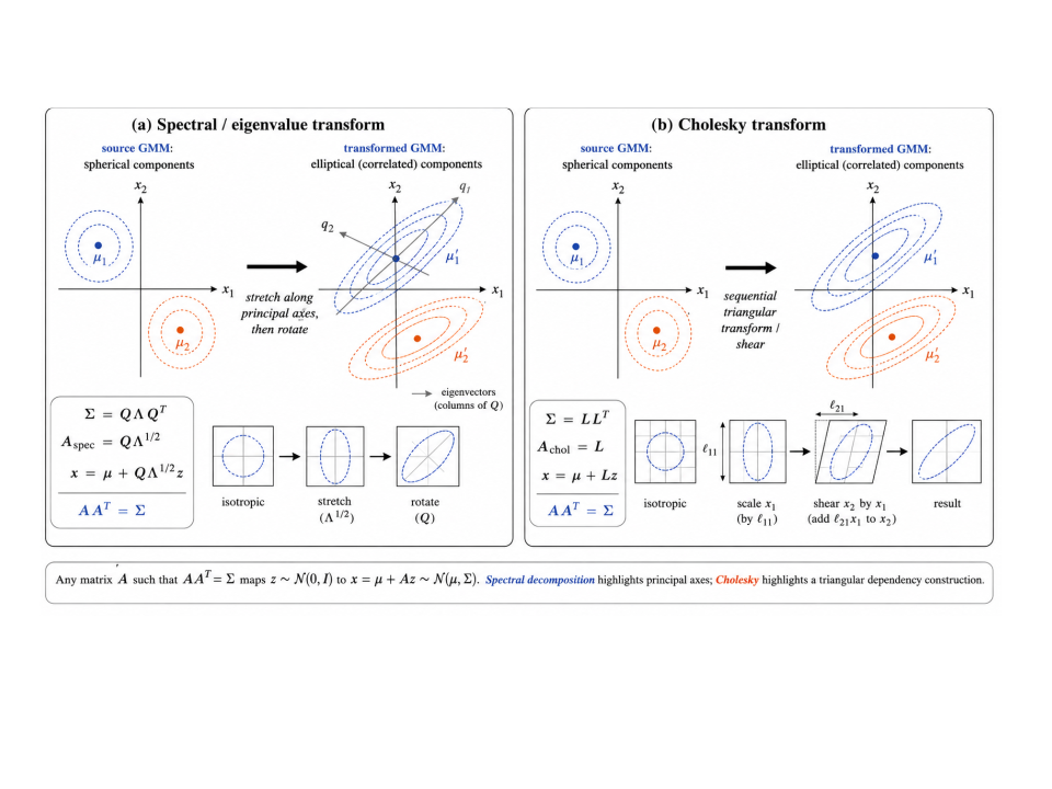
Figure 2 compares the symmetric square root used here with the lower-triangular Cholesky factor of the same R. Both are matrix square roots; they differ by an orthogonal transformation of the coordinate axes, which is exactly the Gram uniqueness (realisations are unique up to orthogonal maps of the ambient space).

Figure 2: Symmetric (spectral) square root versus Cholesky factor of a target Gram. Left: R^{1/2} is symmetric and rotates the standard basis into an eigenframe. Right: the Cholesky factor L with R=LL^{\mathsf{T}} is lower triangular, so the first coordinate is aligned with the first cell type and later types pick up successive residuals. The two embeddings differ by an orthogonal transformation and realise the same pairwise cosines.

The common-factor blend of a shared unit \boldsymbol{u} with private marker blocks (the previous default, closest to AutoGeneS (Aliee and Theis 2021)) is recorded in Sec. 3.3.1. It does not hit \rho exactly at finite J. Cholesky as a Monte Carlo device is in Sec. 3.3.

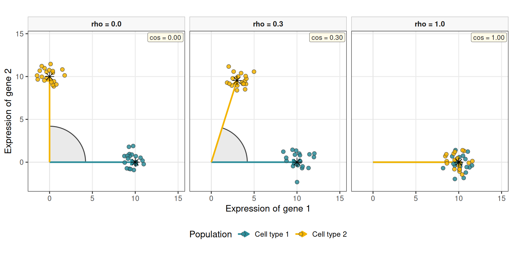
Figure 3 visualises three operating points (\rho\in\{0,\,0.3,\,1\}) for G=2 genes and J=2 cell types. Cell type 1 is fixed along the positive gene-1 axis; only the angular position of cell type 2 is varied so that \rho=0 is exactly orthogonal. Independent Gaussian noise is added only in this vignette chunk around each centroid (N=20 i.i.d. draws per population) to emulate within-type dispersion under an independence assumption, without altering the Gram-matrix generator. Coloured arrows mark each type’s mean direction; the shaded wedge is the angle between the two means.

This illustration is inspired by panel B in the AutoGeneS paper (Aliee and Theis 2021). It is a geometric toy for the target angle, not a plot of Eq. 2: with G=J=2 the symmetric root and the polar construction coincide up to a rotation.

Figure 3: Cosine-control toy for J=2 cell types and G=2 genes. Cell type 1 is fixed on the positive gene-1 axis; only the angular position of cell type 2 varies (so \rho=0 is orthogonal). Coloured arrows: mean directions; shaded wedge: angle between means. Labels report the realised cosine. Points are N=20 i.i.d. Gaussian draws around each centroid (stars). Styling inspired by panel B of AutoGeneS (Aliee and Theis (2021)).

Note 2: Related signature constructions

Blending a common baseline with type-specific markers is standard in deconvolution benchmarking. AutoGeneS (Aliee and Theis 2021) selects genes by jointly minimising inter-type correlation and maximising centroid distance; its simulations use a similar shared-plus-private logic to control signature geometry. Schelker and colleagues (Schelker et al. 2017) build tumour-derived reference gene expression profiles from single-cell RNA-seq clusters and marker genes, then simulate bulk mixtures by combining those columns—empirically a shared baseline plus distinct marker programmes per immune cell type.

The DICEPro framework (Ba et al. 2026) targets incomplete reference matrices in supervised deconvolution. Its simulation engine generates synthetic signature matrices from multivariate Gaussian (or Poisson) models with a prescribed correlation structure; a bloc=TRUE option enforces block sparsity by zeroing expression outside type-specific gene blocks—the common-factor construction of Sec. 3.3.1. DICEPro then optimises reference signatures when cell types are missing from the matrix, complementing the Gram R we use here for method comparison under known ground truth.

Objectives: compute_mean_profile_objectives()

For columns of \boldsymbol{\mu},

\overline{\lvert\cos\rvert} = \frac{2}{J(J-1)} \sum_{1\le j<k\le J} \Biggl| \frac{ \boldsymbol{\mu}_{\cdot j}^{\mathsf{T}} \boldsymbol{\mu}_{\cdot k} }{ \|\boldsymbol{\mu}_{\cdot j}\|_2\, \|\boldsymbol{\mu}_{\cdot k}\|_2 } \Biggr|,

D_{\mathrm{Euc}} = \sum_{1\le j<k\le J} \|\boldsymbol{\mu}_{\cdot j}-\boldsymbol{\mu}_{\cdot k}\|_2.

AutoGeneS treats the first as a quantity to minimise and the second as a quantity to maximise (Aliee and Theis 2021). Cosine is preferred to Pearson correlation so that collinear but unequally scaled profiles remain penalised.

Note 3: Perspectives: a single geometric score for \boldsymbol{\mu}

The present API exposes two AutoGeneS-style objectives. A natural refinement is to replace them by one scalar that jointly rewards large column norms (and hence Euclidean separation) and penalises alignment.

Two candidates are immediate. The Gram determinant

V(\boldsymbol{\mu}) = \sqrt{ \det\bigl( \boldsymbol{\mu}^{\mathsf{T}}\boldsymbol{\mu} \bigr) } \tag{3}

is the volume of the parallelepiped spanned by the columns of \boldsymbol{\mu}. It vanishes under exact collinearity and grows when columns lengthen or become more orthogonal—precisely the desired MOO trade-off in one number.

Equivalently, the reciprocal condition number

\kappa_2(\boldsymbol{\mu})^{-1} = \frac{\sigma_{\min}(\boldsymbol{\mu})}{\sigma_{\max}(\boldsymbol{\mu})}, \tag{4}

available in R via kappa(mean_profiles, exact = TRUE) (or 1 / kappa(...)), measures how ill-posed linear recovery of \boldsymbol{p} from \boldsymbol{y}\approx\boldsymbol{\mu}\boldsymbol{p} is. Maximising \kappa_2(\boldsymbol{\mu})^{-1} (or minimising \kappa_2(\boldsymbol{\mu})) collapses cosine and distance into a deconvolution-centric criterion without a Pareto front.

A practical next step is to expose an optional mean_objective = c("autogenes", "volume", "condition") in simulate_hierarchical_grn_moments(), keep the constructive Gram generator for controllable scenarios, and report the chosen scalar alongside the existing pairwise diagnostics.

Appendix: Cholesky, uniqueness, and the common-factor blend

Cholesky’s factor R=LL^{\mathsf{T}} is the classical Monte Carlo square root: if \boldsymbol{z} is standard normal, L\boldsymbol{z} has covariance R (Madar 2015). The same factor embeds J unit vectors as the rows of L (padded by zeros in \mathbb{R}^{G}). The first type is aligned with the first coordinate; later types pick up successive residuals, so the embedding is order-dependent. The symmetric root R^{1/2} has no preferred axis. Figure 2 is that distinction. Vector realisations of a Gram matrix are unique only up to an orthogonal map of the ambient space: if \boldsymbol{\mu}^{\mathsf{T}}\boldsymbol{\mu}=s^{2}R, so is (\mathbf{Q}\boldsymbol{\mu})^{\mathsf{T}} (\mathbf{Q}\boldsymbol{\mu}) for \mathbf{Q}^{\mathsf{T}}\mathbf{Q}= \mathbf{I}. Equicorrelation Grams used as target_cosine are double-constant matrices (O’Neill 2021); Mustonen’s total-variability scalar is a related summary of a multivariate Gaussian covariance, not a substitute for the Gram construction (Mustonen 1997).

Common-factor construction

The previous package default blended a shared unit \boldsymbol{u}=G^{-1/2}\mathbf{1} with private, disjoint marker blocks \boldsymbol{v}_{j},

\tilde{\boldsymbol{\mu}}_{\cdot j} = \sqrt{\rho}\,\boldsymbol{u} +\sqrt{1-\rho}\,\boldsymbol{v}_{j}, \tag{5}

then column-normalised. Because \boldsymbol{u} is not orthogonal to the blocks, the realised cosine exceeds \rho at finite J. That construction remains the closest analogue of AutoGeneS shared-plus-private geometry (Aliee and Theis 2021); the default generator is now Eq. 2, which hits R exactly.

Undirected Gaussian Markov network generation

G \longrightarrow W(G) \longrightarrow \Omega \succ 0 \longrightarrow X_i \sim \mathcal{N}_p(\mu_i,\Omega^{-1}) \tag{6}

Here G is an undirected graph, W(G) a symmetric weighted matrix with the same off-diagonal support, \Omega a strictly positive-definite precision, and X_i an expression profile. This section covers undirected Gaussian Markov / precision-graph simulation only. generate_random_network_skeleton() draws G; build_normalised_precision() completes it to \Omega\succ 0 by an affine spectral shift; build_covariance_array_from_precision() maps each slice \boldsymbol{\Sigma}_j=\boldsymbol{\Omega}_j^{-1} (cell types need not share one network).

%%{init: {"theme": "sandstone"}}%%
flowchart LR
  G["Undirected graph G"] --> W["Signed weights W(G)"]
  W --> Omega["SPD precision Ω"]
  Omega --> Latent["Latent Gaussian X"]
  Mu["Mean design μ"] --> Latent
  Latent --> Obs["Observation layer"]

Figure 4: Undirected simulation pipeline from topology to observations (optional observation layer dashed).

Graph structure generators

\rho_{jk\mid -\{j,k\}} = -\frac{\Omega_{jk}}{\sqrt{\Omega_{jj}\Omega_{kk}}} \tag{7}

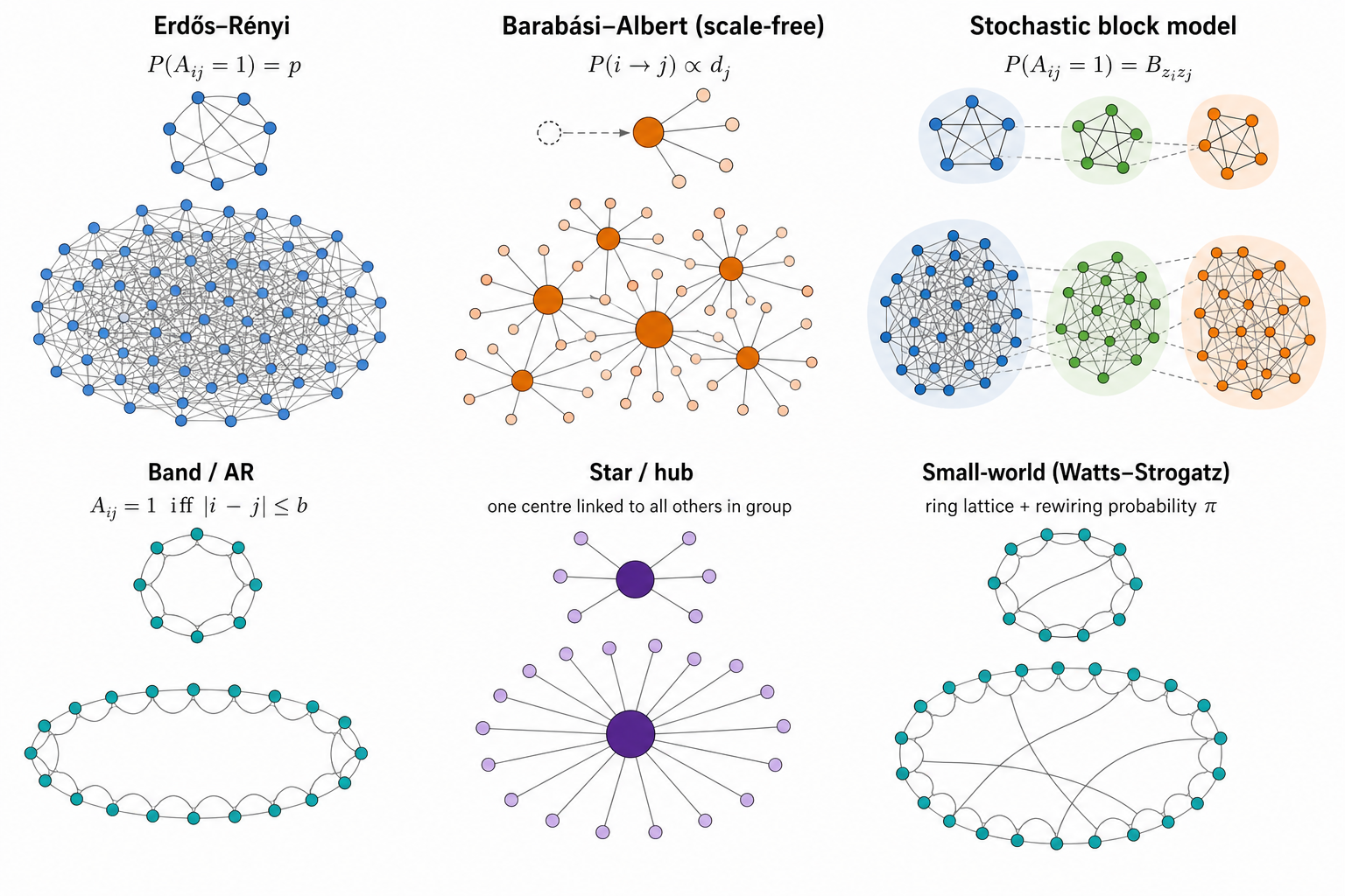
Table 1 compares the main undirected topology families used in GGM benchmarks, with R entry points. Figure 5 sketches the six families most often used in random-like network structure generation.

Table 1: Topology families for undirected GGM simulation (R-focused).

Structure	Definition and controls	R entry points	Advantages	Limitations
Erdős–Rényi	Each edge present independently with probability q; q=d_{\mathrm{avg}}/(p-1) targets average degree	huge::huge.generator(graph="random") (Jiang et al. 2026); BDgraph::graph.sim(graph="random") (Mohammadi and Wit 2025); DeCovarT graph_model = "erdos_renyi"	Exact sparsity control in expectation; few nuisance parameters	Narrow degree distribution; little modular organisation
Band / AR	Edge j–k if 1\le\lvert j-k\rvert\le b	huge.generator(graph="band") (Jiang et al. 2026); BDgraph::bdgraph.sim(graph="AR(1)") / "AR(2)" (Mohammadi and Wit 2025)	Local dependence and controlled max degree	Artificial gene ordering; no hubs or modules
Hub / star	g groups; one centre linked to remaining members	huge.generator(graph="hub") (Jiang et al. 2026); graph.sim(graph="hub") / "star" (Mohammadi and Wit 2025); DeCovarT graph_model = "hub"	Stress-tests high-degree regulators	Pure stars omit cross-talk
Scale-free	Preferential attachment (e.g. Barabási–Albert with m edges per new node)	huge.generator(graph="scale-free") (Jiang et al. 2026); DeCovarT graph_model = "scale_free"	Heterogeneous degrees	Weak modularity under plain BA growth
Cluster / SBM	Within-block edge probability exceeds between-block (Holland et al. 1983)	huge.generator(graph="cluster") (Jiang et al. 2026); DeCovarT graph_model = "stochastic_block_model"	Pathway / module structure	Equal blocks can be unrealistically regular
Small-world / lattice / circle	High clustering with short paths, or fixed neighbourhoods (Watts and Strogatz 1998)	DeCovarT graph_model = "small_world" (Watts–Strogatz); BDgraph::graph.sim(graph="smallworld") (Mohammadi and Wit 2025)	Local modules and spatial organisation	Narrow degrees; needs a defensible ordering

Figure 5: Six undirected topology families used in GGM simulation: Erdős–Rényi, Barabási–Albert (preferential attachment / scale-free), stochastic block (cluster), band / AR, star / hub, and small-world (Watts–Strogatz).

Not every topology is equally useful as a gene-regulatory prior. The three simulation studies in Table 3, together with classical network biology, suggest the following reading.

Table 2: Biological interpretability of undirected topology families.

Family	Biological reading	Why it matters for DeCovarT
Star / hub	Master-regulator TF with many targets; one-to-many signalling	Stress-tests recovery of a few high-degree hubs that dominate partial correlations (Wu and Luo 2022; Federico et al. 2023)
Scale-free (BA)	Preferential attachment produces a heavy-tailed degree distribution and several hubs (Barabási and Albert 1999)	Standard high-dimensional GGM stress test used by SILGGM via huge (Zhang et al. 2018); useful for testing degree heterogeneity, but not a default empirical model of gene regulation
Cluster / SBM	Co-regulated modules / pathways with dense within-block links (Holland et al. 1983)	Matches pathway organisation; BLGGM’s global block partition is SBM-like before finer within-block motifs (Wu and Luo 2022)
Small-world	High local clustering with short paths (ring + shortcuts) (Watts and Strogatz 1998)	Local co-expression neighbourhoods plus long-range regulatory shortcuts; useful when modularity is soft rather than hard blocks (Federico et al. 2023)
Band / AR	Ordered local dependence only	Useful numerical control, but gene indices rarely encode a natural order—limited biological fidelity (Zhang et al. 2018)
Erdős–Rényi	Homogeneous random wiring	Null / baseline sparsity; little pathway or hub structure (Zhang et al. 2018)

Note 4: The scale-free hypothesis: a useful stress test, not a biological default

The phrase scale-free network usually means that the degree distribution follows a power law, \Pr(K=k)\propto k^{-\alpha}, at least above a lower cut-off. This statistical statement is distinct from the Barabási–Albert (BA) growth mechanism. Preferential attachment can generate a power law, but observing a heavy-tailed degree distribution does not establish preferential attachment; other mechanisms can produce similar tails, and variants of preferential attachment need not produce a pure power law (Lima-Mendez and van Helden 2009; Broido and Clauset 2019).

Whether biological networks are scale-free has therefore remained contested. Early claims often relied on approximately straight log–log degree plots. Such plots are not goodness-of-fit tests: binning, the plotting scale, a small number of hubs, and incomplete or biased sampling can all make non-power-law distributions appear linear. The underlying graph representation matters as well. For example, pool metabolites can become artificial hubs in metabolic graphs, while protein-interaction networks depend strongly on the assay and sampling scheme (Lima-Mendez and van Helden 2009). A power law should instead be fitted to the discrete degree data, tested for plausibility, and compared on the same support with alternatives such as log-normal, exponential, stretched-exponential, and power-law-with-cut-off distributions.

The evidence is not uniformly negative. Using adjacency-spectrum distributions rather than degree alone, Takahashi and colleagues classified eight protein–protein interaction networks as scale-free (Takahashi et al. 2012). Importantly, this was a relative model-selection result: BA-like networks fitted better than the two candidate alternatives, Erdős–Rényi and Watts–Strogatz networks. It did not show that a power law was an adequate absolute model, that preferential attachment generated the observed networks, or that unobserved interactions would preserve the classification. The authors explicitly noted both the restricted candidate set and possible sampling artefacts.

A broader test of 928 real-world network data sets reached a more cautious conclusion (Broido and Clauset 2019). Across all domains, only 4% met the strongest scale-free criterion, whereas a log-normal distribution fitted as well as or better than a power law for 88% of degree distributions. Among the biological networks, 63% showed neither direct nor indirect evidence of scale-free structure, although 6% met the strongest criterion, principally metabolic networks. These proportions depend on the network corpus and the operational definition of scale-freeness, but they reject a universal scale-free law rather than excluding scale-free structure from every biological system.

Table 3 summarises how recent simulation studies combine topology, precision construction, and mean / observation models.

Table 3: Literature survey of undirected graph → precision → observation designs.

Source	Graph structures	Precision construction	Mean / observation	Purpose
PLNnetwork (Chiquet et al. 2018)	Erdős–Rényi, preferential attachment, affiliation	\Omega = vG + \operatorname{diag}(\lvert\lambda_{\min}(vG)\rvert + u)	Latent log-abundance XB; compositional / multinomial counts	Count-network estimators under compositionality
SILGGM (Zhang et al. 2018)	Band, hub, Erdős–Rényi, scale-free via huge	Package covariance / precision simulation	Centred Gaussian; focus on precision entries	Large-p inferential and computational stress tests
BLGGM (Wu and Luo 2022)	Block mixtures of dense, circle, star, signed modules	Module matrices with structured signed off-diagonals	Cell-type-specific \mu_k, \Omega_k; expression-dependent dropout	Joint clustering, heterogeneous networks, zero inflation

Several conclusions follow.

1. Band is not intrinsically a random-graph model: its support is usually deterministic once the bandwidth is fixed. Hub constructions are often partly deterministic as well. Erdős–Rényi, preferential attachment, and stochastic block models are genuinely stochastic.
2. A positive off-diagonal entry in \Omega encodes a negative partial correlation (Eq. 7). Uniformly positive precision weights therefore induce uniformly negative edgewise partial correlations; random or signed biological weights are needed when activation-like and inhibition-like associations matter.
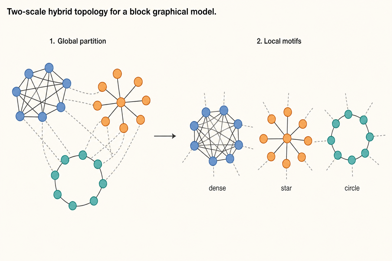
3. BLGGM is a two-scale hybrid (Wu and Luo 2022), shown in Figure 6:
   • Global partition. Genes are assigned to blocks (a stochastic-block–like cut); between-block edges are sparse.
   • Local motifs. Inside each block the topology can be a dense clique, a circle, a star / hub, or a signed dense module, so distinct blocks can stand for distinct regulatory regimes (co-expression programmes, cyclic motifs, master-regulator hubs). Signs may differ across modules or cell types.
   The construction remains fully undirected, but it is richer than a flat Erdős–Rényi draw. DeCovarT’s exported generators currently expose the three families most useful as standalone benchmarks: scale_free, stochastic_block_model, and small_world.

Figure 6: Two-pronged BLGGM-style topology: a global stochastic-block partition of genes, then a local motif (dense module, star, or circle) inside each block (Wu and Luo 2022).

Weight design and random signs

Topology generators return a binary undirected support E. Signs and magnitudes are a separate design layer W(G) in Eq. 6: they are assigned after (or jointly with) the skeleton, then completed to an SPD precision. Remember that

\operatorname{sign}(\rho_{jk\mid -\{j,k\}}) = -\operatorname{sign}(\Omega_{jk}) \tag{8}

see Eq. 7, so a positive precision weight is an inhibitory partial correlation. Table 4 contrasts three standard undirected strategies.

Table 4: Three undirected strategies for signed / random edge weights after a fixed skeleton.

Approach	What is randomised	How \Omega is obtained	When to use
i.i.d. edge signs	For each \{j,k\}\in E, draw s_{jk}\in\{-1,+1\} (e.g. fair coin or \mathbb{P}(+)=\pi) and magnitude m_{jk}>0; set W_{jk}=W_{kj}=s_{jk}m_{jk}	Support-preserving SPD map of W (spectral shift, diagonal dominance, …)	Simple signed ER / hub / SBM benchmarks; explicit control of the inhibitory fraction
Partial-correlation scaling	Fill a symmetric matrix R with R_{jk}=0 off E and R_{jk}\in(-1,1) (signed) on E; ensure \rho(R)<1	\Omega = D^{1/2}(I-R)D^{1/2} (Eq. 11)	Direct control of partial-correlation signs and strengths
G-Wishart (BDgraph::rgwish())	Continuous random \Omega on the fixed graph zeros	\Omega\sim W_G(b,D) already SPD (Mohammadi and Wit 2025, 2019)	Heterogeneous random weights without hand-tuned magnitudes; Bayesian-style replicates

i.i.d. signs on a fixed skeleton

Draw G (ER, band, hub, …). Independently for each undirected edge,

W_{jk}=W_{kj}=s_{jk}\,m_{jk}, \qquad s_{jk}\in\{-1,+1\}, \quad m_{jk}>0, \tag{9}

then apply a support-preserving SPD completion (next section). Uniform positive loadings W=vG are the special case s_{jk}\equiv +1 used by PLN-style and many huge simulations (Chiquet et al. 2018)—all partial correlations then share the same sign. DeCovarT uses i.i.d. signs with inhibitory fraction prop_inhibitory and magnitude v (precision_scale) baked into \boldsymbol{W} before the spectral SPD completion.

Partial-correlation scaling and why I-R

In a Gaussian Markov model the matrix of partial correlations (with ones on the diagonal) relates to the precision by a diagonal congruence. Write the off-diagonal partial correlations as a symmetric matrix R with

R_{jj}=0, \qquad R_{jk} = \begin{cases} \rho_{jk\mid -\{j,k\}} & \{j,k\}\in E,\\ 0 & \{j,k\}\notin E, \end{cases} \tag{10}

and choose magnitudes so that the spectral radius satisfies \rho(R)<1. Then

\Omega = D^{1/2}(I-R)D^{1/2} \tag{11}

for a positive diagonal D (often D=I after standardising margins).

G-Wishart draws on a fixed graph

Given adjacency G, BDgraph::rgwish() samples \Omega\sim W_G(b,D) already positive definite and with \Omega_{jk}=0 whenever (j,k)\notin E (Mohammadi and Wit 2025, 2019). Signs and magnitudes arise from the continuous distribution rather than from an explicit coin-flip layer. This is the most “automatic” signed-weight generator once the skeleton is fixed; the trade-off is less direct control of the inhibitory fraction than Eq. 9 or Eq. 11.

Positive-definiteness strategies

Table 5 contrasts constructions that turn a weighted support W (or a partial-correlation design) into \Omega\succ 0. DeCovarT’s build_normalised_precision() implements the uniform spectral shift below, with diagonal cushion u (precision_shift):

\boldsymbol{\Omega} = \boldsymbol{W} + \bigl( \lvert\lambda_{\min}(\boldsymbol{W})\rvert + u \bigr) \mathbf{I}.

Table 5: Support-preserving maps from a weighted graph to \Omega\succ 0. Eigenvalue clipping (reconstruct Q\Lambda_{\mathrm{clip}}Q^{\top}) fills structural zeros, so it is omitted from the generative truth; nearest-PD projections are repair tools, not support-preserving simulators.

Construction	Formula	Support preserved?	Role
Spectral / PLN loading	\Omega=W+(\lvert\lambda_{\min}(W)\rvert+u)I	Yes	DeCovarT default; same affine shift as huge / PLN (Chiquet et al. 2018)
Partial-correlation scaling	\Omega=D^{1/2}(I-R)D^{1/2}, \rho(R)<1	Yes	Signs and strengths set on the partial-correlation scale (Eq. 11)
Graph Laplacian / M-matrix	\Omega=L_G+\varepsilon I	Yes	Off-diagonals non-positive ⇒ all edgewise partial correlations positive
G-Wishart	\Omega\sim W_G(b,D)	Yes	Heterogeneous random weights; BDgraph::rgwish() (Mohammadi and Wit 2025)

Why the uniform spectral shift is attractive

If W=Q\Lambda Q^{\top}, then (Eq. 12)

W+cI = Q(\Lambda+cI)Q^{\top}. \tag{12}

Every eigenvalue increases by c, while every off-diagonal of W is unchanged, so the edge set

E=\{(j,k):j<k,\ \Omega_{jk}\neq 0\} \tag{13}

is identical before and after loading—and signs of W are preserved.

The floor \varepsilon also controls the condition number

\kappa(\Omega)=\frac{\lambda_{\max}(\Omega)}{\lambda_{\min}(\Omega)}. \tag{14}

Large loading yields a well-conditioned but weakly dependent network; loading only slightly above -\lambda_{\min} strengthens dependence but can make estimation fragile. Benchmarks should report partial-correlation distributions and \kappa(\Omega), not only the adjacency.

If a Cholesky factor of \boldsymbol{\Omega} still fails after this loading, build_normalised_precision() repeats the same affine shift with a larger u until \boldsymbol{\Omega}\succ 0 strictly. If \boldsymbol{\Sigma}=\boldsymbol{\Omega}^{-1} then fails to factor—typical of hub graphs with a tiny u—simulate_hierarchical_grn_moments() (and build_covariance_array_from_precision()) increases that same diagonal loading on \boldsymbol{\Omega} until both matrices are strictly positive definite. Off-diagonal support and signs of W are unchanged.

Cell-type covariances: build_covariance_array_from_precision()

By default each cell type has its own precision (and thus covariance),

\boldsymbol{\Sigma}_j = \boldsymbol{\Omega}_j^{-1}, \qquad j=1,\ldots,J,

stacked as an array in \mathcal{M}_{G\times G\times J}. Shared networks remain available by supplying the same adjacency (or the same graph model seed path) for every type.

Note 5: Why the bulk covariance is \sum_j p_j^{2}\boldsymbol{\Sigma}_j

If each latent profile is \boldsymbol{x}_{\cdot j}\sim\mathcal{N}_{G}(\boldsymbol{\mu}_{\cdot j},\boldsymbol{\Sigma}_j) independently, the bulk \boldsymbol{y}=\sum_j p_j\boldsymbol{x}_{\cdot j} is an affine image of a stacked Gaussian vector. Affine images of multivariate Gaussians remain Gaussian, with mean \boldsymbol{\mu}\boldsymbol{p} and covariance \sum_j p_j^{2}\boldsymbol{\Sigma}_j (the p_j^{2} factor is the square of the linear coefficient, not a mixture-weight identity). That is the conditional law used in the article (Gaussian convolution with covariance \sum_j p_j^{2}\boldsymbol{\Sigma}_j; see the log-likelihood derivation in article/main.tex) and by simulate_bulk_mixture(). Downstream bulk simulation therefore uses

\boldsymbol{y}\mid(\boldsymbol{\zeta},\boldsymbol{p}) \sim \mathcal{N}_{G}\bigl(\boldsymbol{\mu}\boldsymbol{p}, \textstyle\sum_j p_j^{2}\boldsymbol{\Sigma}_j\bigr).

Imbalanced cellular proportions

Topology and mean design fix the reference moments \boldsymbol{\zeta}. Mixture difficulty also depends on how uneven the true composition \boldsymbol{p} is. DeCovarT summarises that imbalance with the normalised Shannon entropy compute_shannon_entropy(),

H^{\star}(\boldsymbol{p}) = \frac{-\sum_{j:p_{j}>0}p_{j}\log p_{j}}{\log J} \in[0,1], \tag{15}

so H^{\star}=0 for a Dirac mass on one type and H^{\star}=1 for the uniform vector on J types. Zero masses are dropped only inside the sum; the normaliser still uses the full panel size J.

A practical grid therefore crosses network / mean axes with a few composition designs, for example:

Table 6: Composition designs scored by normalised Shannon entropy.

Design	Example \boldsymbol{p} (up to permutation)	Typical H^{\star}
Pure / near-pure	(1,0,\ldots) or (0.95,0.05,0,\ldots)	near 0
One dominant type	(0.7,0.15,0.15)	low–moderate
Two-way balance	(0.5,0.5) or (0.4,0.4,0.2)	moderate–high
Uniform	(1/J,\ldots,1/J)	1

The Bioconductor package SimBu (Dietrich 2024) offers a complementary pseudo-bulk toolkit with six named fraction scenarios (even, random, mirror_db, weighted, pure, custom) when aggregating single-cell profiles; see the SimBu “Simulate pseudo bulk datasets” section. Figure 7 shows five of those designs for J=6 types as stacked compositions, labelled by H^{\star}(\boldsymbol{p}). High-entropy (even) mixtures spread mass across types; low-entropy (pure) mixtures collapse onto one type. DeCovarT’s Gaussian convolution uses the same idea at the moment layer: supply p (or a J\times N matrix of sample-wise ratios) to simulate_bulk_mixture(), and report H^{\star} alongside overlap or condition-number diagnostics. The hybrid J=3 manuscript scenario uses composition_from_entropy() at H^{\star}\in\{1,0.5,0.1\} (covariance-driven hybrid).

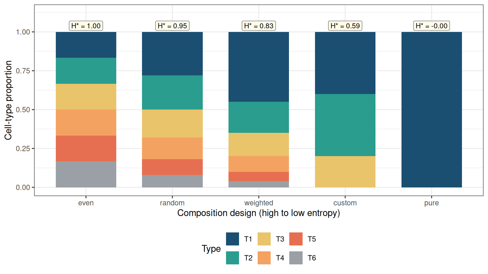
Figure 7: Illustrative J=6 compositions spanning SimBu-style fraction scenarios, ordered by decreasing normalised Shannon entropy H^{\star}(\boldsymbol{p}). Each bar is one design; geom_label reports H^{\star}. mirror_db is omitted (it copies an empirical atlas rather than a fixed simplex vector).

Scenario descriptors collected with the bulk draw

describe_simulation_scenario() records the convolution parameters (\boldsymbol{p},\boldsymbol{\mu},\{\boldsymbol{\Sigma}_j\}) and a compact geometry table. run_simulation_benchmark() returns those objects as theta_true, descriptors, supplementary, and call (match.call()). Kept measures stay in six families (Note 6, Note 7, Note 9, Note 10, Note 11, Note 12). MixSim BarOmega and averaged pairwise Hellinger of the purified Gaussians summarise the same convolution components as the bulk law, so they sit in descriptors. Jeffreys / symmetrised KL is stored in supplementary. There is no composite global score: each column answers a different question.

Compositions on a Shannon grid can be built with composition_from_entropy() (one-dominant family (1-(J-1)q,q,\ldots,q) matching a target H^{\star}).

Table 7: Kept scenario descriptors from describe_simulation_scenario() (R/02_03_scenario_descriptors.R). Jeffreys sits on the same ID key in supplementary / the descriptors RDS.

Metric	Formula	Bounds	Captures	Pros_cons
Composition	Composition	Composition	Composition	Composition
Normalised Shannon entropy (h_star)	\(H^{\star}=H(p)/\log J\)	\([0,1]\)	Evenness of \(p\) (Pielou); \(0\) is a vertex	\(J\)-normalised. Zeros use \(0\log 0=0\).
Effective number (n_eff)	\(n_{\mathrm{eff}}=\exp\{H(p)\}\)	\([1,J]\)	Hill number of order \(1\)	Interpretable count. Not a probability.
Active count (n_active)	\(\#\{j:p_j>\varepsilon\}\)	\(\{0,\ldots,J\}\)	Simplex stratum (how many types are on)	Threshold \(\varepsilon\) is a convention.
Concentration \(\lVert p\rVert_2^2\)	\(\sum_j p_j^2\)	\([1/J,1]\)	Weight in \(\Sigma(p)=\sum_j p_j^2\Sigma_j\)	Directly scales \(\Sigma(p)\). Ignores means.
Mean geometry	Mean geometry	Mean geometry	Mean geometry	Mean geometry
Mean absolute cosine	\(J^{-1}\sum_{j<k}\lvert\cos(\mu_{\cdot j},\mu_{\cdot k})\rvert\)	\([0,1]\)	Typical mean-profile confusion	Scale-free. Misses Euclidean gaps.
Highest pairwise cosine (max_cosine)	\(\max_{j<k}\cos(\mu_{\cdot j},\mu_{\cdot k})\)	\([-1,1]\)	Worst pair of collinear signatures	Safety diagnostic for two-type confusion.
Mean Euclidean gap (mean_euclidean)	mean of \(\lVert\mu_{\cdot j}-\mu_{\cdot k}\rVert_2\)	\([0,\infty)\)	Centroid (CLD) separation in \(\mathbb{R}^G\)	Matches the article CLD factor. Not Aitchison.
Condition number \(\kappa(\mu)\)	\(\sigma_{\max}(\mu)/\sigma_{\min}(\mu)\)	\([1,\infty]\)	Near-collinearity of the signature frame	Sensitive to a single tiny singular value.
Gram volume	\(\prod_\ell \sigma_\ell(\mu)\)	\([0,\infty)\)	Volume of the parallelepiped; \(0\) at rank loss	Product of singular values; units of \(\mu\).
SPD / \(\Sigma(p)\)	SPD / \(\Sigma(p)\)	SPD / \(\Sigma(p)\)	SPD / \(\Sigma(p)\)	SPD / \(\Sigma(p)\)
\(\lambda_{\min}\{\Sigma(p)\}\)	smallest eigenvalue of \(\Sigma(p)\)	\([0,\infty)\)	Distance of the bulk covariance to singularity	Numerical, not statistical, identifiability.
kappa_sigma_p	\(\lambda_{\max}/\lambda_{\min}\)	\([1,\infty]\)	Anisotropy of the bulk ellipsoid	Flags Cholesky / log-det instability.
kappa_sigma_reciprocal	\(\lambda_{\min}/\lambda_{\max}\in(0,1]\)	\((0,1]\)	The same ratio on a bounded scale	Easier to plot than \(\kappa\).
Tangent Fisher	Tangent Fisher	Tangent Fisher	Tangent Fisher	Tangent Fisher
\(\lambda_{\min}(I_T)\)	weakest Helmert contrast of \(I\)	\([0,\infty)\)	Weakest identifiable simplex contrast	Local information, not finite-sample RMSE.
\(\kappa(I_T)\)	\(\lambda_{\max}(I_T)/\lambda_{\min}(I_T)\)	\([1,\infty]\)	Ill-posed directions on the simplex	Large \(\kappa\) hides one easy contrast.
\(f_{\mathrm{cov}}\)	\(\mathrm{tr}(I^{\mathrm{cov}})/\mathrm{tr}(I)\)	\([0,1]\)	Share of Fisher information from covariance	Near \(1\), LSEI / CIBERSORT are under-informed.
\(f_{\mathrm{cov}}^{\max}\)	max of that fraction on \(e_j-e_k\)	\([0,1]\)	Worst pairwise contrast for mean-only solvers	Same interpretation on the hardest pair.
Network sparsity	Network sparsity	Network sparsity	Network sparsity	Network sparsity
Edge density / mean degree	\(2\lvert E\rvert/(G(G-1))\); \(2\lvert E\rvert/G\)	\([0,1]\); \([0,G-1]\)	Binary graph density (or precision support)	For fixed \(G\), density and mean degree match.
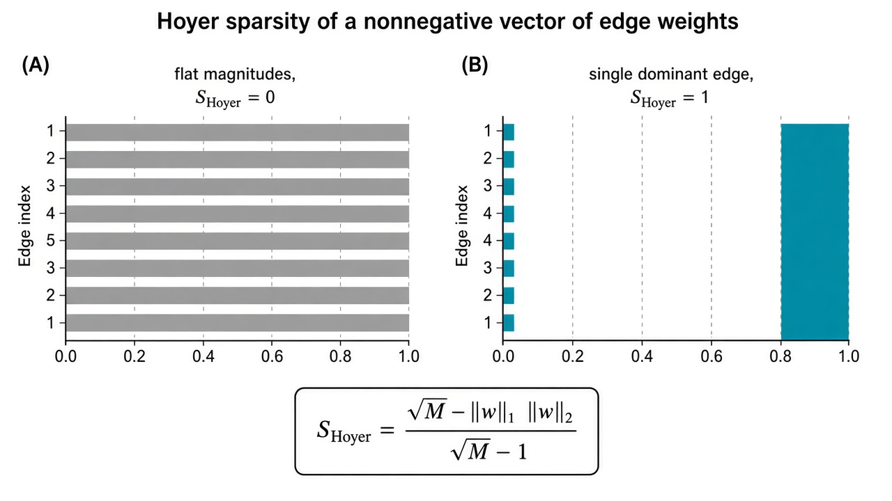
Hoyer sparsity of \(\lvert r_{gh}\rvert\)	\((\sqrt{M}-\lVert w\rVert_1/\lVert w\rVert_2)/(\sqrt{M}-1)\)	\([0,1]\)	Magnitude sparsity of bulk correlations	Scale-free; no topology assumed.
Component overlap	Component overlap	Component overlap	Component overlap	Component overlap
MixSim BarOmega	average pairwise misclassification	\([0,1]\)	Overlap of the \(J\) purified Gaussians	Davies for \(G<4\); Sobol Monte Carlo otherwise.
Mean pairwise Hellinger	\(J^{-1}\sum_{j<k} H_2(f_j,f_k)\) (symmetric)	\([0,1]\)	Symmetric affinity of those Gaussians	Closed form; \(H_2(f,g)=H_2(g,f)\).
Mean pairwise AIRM (riemannian_sigma)	mean of \(d_R(\Sigma_j,\Sigma_\ell)\)	\([0,\infty)\)	SPD geodesic gap of the \(\Sigma_j\) (not Frobenius)	Inversion-invariant; infinite at singularity.
Supplementary	Supplementary	Supplementary	Supplementary	Supplementary
Jeffreys / symmetrised KL	\(\tfrac12\mathrm{KL}(f\|g)+\tfrac12\mathrm{KL}(g\|f)\)	\([0,\infty)\)	Symmetrised KL of the same pair average	Not a metric; recorded separately.

Note 6: Composition

Let \boldsymbol{p}\in\Delta^{J-1} with the convention 0\log 0=0. The normaliser always uses the full panel size J, including zeros.

• Normalised Shannon entropy H^{\star}(\boldsymbol{p})=H(\boldsymbol{p})/\log J, H(\boldsymbol{p})=-\sum_j p_j\log p_j. Zero is a Dirac mass; one is the uniform composition.
• Effective number of types n_{\mathrm{eff}}=\exp\{H(\boldsymbol{p})\}. Equals J at the barycentre and 1 at a vertex.
• Active count n_{\mathrm{active}}=\#\{j:p_j>\varepsilon\} and \min_j p_j among active components: simplex stratum and distance to a face.
• Concentration \sum_j p_j^2=\lVert\boldsymbol{p}\rVert_2^2. This is the weight that scales the convolution covariance \boldsymbol{\Sigma}(\boldsymbol{p})=\sum_j p_j^2\boldsymbol{\Sigma}_j.

Note 7: Mean geometry

Columns of \boldsymbol{\mu} are built by generate_mean_signature_matrix() so that the Gram of unit columns equals target_gram (or equicorrelation at target_cosine). Euclidean gaps then scale with mean_scale s: \lVert\boldsymbol{\mu}_{\cdot j}-\boldsymbol{\mu}_{\cdot k}\rVert =s\sqrt{2(1-\cos(\boldsymbol{\mu}_{\cdot j},\boldsymbol{\mu}_{\cdot k}))}. Use nonnegative = TRUE for a disjoint-support frame when the downstream solver requires \boldsymbol{\mu}\ge 0.

• Mean absolute pairwise cosine and the highest cosine: which types are confusable from first-order signatures alone.
• Mean pairwise Euclidean gap of the signature columns (the quantity the article labels CLD; see Note 8).
• Condition number \kappa(\boldsymbol{\mu})=\sigma_{\max}/\sigma_{\min} of the singular values of \boldsymbol{\mu}: near-collinearity of the signature parallelepiped.
• Gram volume \prod_{\ell}\sigma_{\ell}(\boldsymbol{\mu}) (zero at rank loss).

Note 8: Euclidean centroid gap (CLD)

CLD is a shorthand for centroid (mean-profile) separation: how far two signature columns \boldsymbol{\mu}_{\cdot 1} and \boldsymbol{\mu}_{\cdot 2} sit in gene space. The article uses the same label (“mean centroids (CLD)”). There is no separate named CLD index in the package; mean_euclidean is the mean of those pairwise gaps, the same Euclidean objective compute_mean_profile_objectives() maximises. The signatures are expression means, not simplex compositions, so this is not an Aitchison / clr distance.

The Euclidean gap, the inner product, and the cosine of the angle \theta are the same geometry (dot product, geometric definition):

\boldsymbol{\mu}_{\cdot 1}^{\mathsf{T}}\boldsymbol{\mu}_{\cdot 2} = \lVert\boldsymbol{\mu}_{\cdot 1}\rVert_2 \lVert\boldsymbol{\mu}_{\cdot 2}\rVert_2 \cos\theta,

d(\boldsymbol{\mu}_{\cdot 1},\boldsymbol{\mu}_{\cdot 2}) = \lVert\boldsymbol{\mu}_{\cdot 1}-\boldsymbol{\mu}_{\cdot 2}\rVert_2 = \sqrt{ \lVert\boldsymbol{\mu}_{\cdot 1}\rVert_2^2 + \lVert\boldsymbol{\mu}_{\cdot 2}\rVert_2^2 - 2\,\boldsymbol{\mu}_{\cdot 1}^{\mathsf{T}}\boldsymbol{\mu}_{\cdot 2} }.

On the bivariate toy the two designed levels are:

Level	\boldsymbol{\mu}_{\cdot 1}	\boldsymbol{\mu}_{\cdot 2}	d	cosine
small CLD	(20,22)	(22,20)	\sqrt{8}=2\sqrt{2}\approx 2.83	880/884\approx 0.995
large CLD	(20,40)	(40,20)	\sqrt{800}=20\sqrt{2}\approx 28.3	0.8

Small CLD means nearly overlapping centroids (harder for mean-only solvers). Large CLD means the two types are well separated in \mathbb{R}^G.

Note 9: SPD / numerical conditioning of \boldsymbol{\Sigma}(\boldsymbol{p})

These columns describe the mixture covariance, not statistical identifiability of \boldsymbol{p}. For a Gaussian, \kappa\{\boldsymbol{\Sigma}(\boldsymbol{p})\} =\lambda_{\max}/\lambda_{\min} =\kappa\{\boldsymbol{\Omega}(\boldsymbol{p})\}.

• \lambda_{\min}\{\boldsymbol{\Sigma}(\boldsymbol{p})\}: distance to a singular convolution covariance.
• kappa_sigma_p \kappa\{\boldsymbol{\Sigma}(\boldsymbol{p})\}=\lambda_{\max}/\lambda_{\min}: anisotropy of the bulk ellipsoid. Large \kappa makes Cholesky, log-determinants, and analytic gradients sensitive.
• kappa_sigma_reciprocal \lambda_{\min}/\lambda_{\max}\in(0,1]: the same ratio on a bounded scale (one is isotropic).

Note 10: Tangent Fisher information (mean versus covariance)

For a real Gaussian \boldsymbol{y}\mid\boldsymbol{p}\sim \mathcal{N}_{G}(\boldsymbol{\mu}\boldsymbol{p},\boldsymbol{\Sigma}(\boldsymbol{p})), the ambient Fisher matrix is the Slepian–Bangs formula with two summands: a Mahalanobis (mean) term and a whitened-Frobenius (covariance) term. McCulloch (McCulloch 1982) derives that split for the multivariate normal by treating \boldsymbol{\Sigma} as symmetric (\mathrm{vech}, not \mathrm{vec}), which supplies the factor \tfrac12 on the covariance block. Besson and Abramovich (Besson and Abramovich 2013) extend Slepian–Bangs to elliptically contoured laws: the two Gaussian terms survive, scaled by expectations of the modular variate; the Gaussian case recovers the original formula.

DeCovarT is that Gaussian special case, with \boldsymbol{p} in both the mean \boldsymbol{\mu}\boldsymbol{p} and \boldsymbol{\Sigma}(\boldsymbol{p})=\sum_j p_j^2\boldsymbol{\Sigma}_j. The two summands therefore mix in every coordinate of I(\boldsymbol{p}). Substituting \partial(\boldsymbol{\mu}\boldsymbol{p})/\partial p_j=\boldsymbol{\mu}_{\cdot j} and \partial\boldsymbol{\Sigma}(\boldsymbol{p})/\partial p_j=2p_j\boldsymbol{\Sigma}_j yields

I_{jk}(\boldsymbol{p}) = \underbrace{ \boldsymbol{\mu}_{\cdot j}^{\mathsf{T}} \boldsymbol{\Omega}(\boldsymbol{p}) \boldsymbol{\mu}_{\cdot k} }_{I^{\mathrm{mean}}_{jk}} + \underbrace{ 2 p_j p_k \operatorname{tr}\bigl( \boldsymbol{\Omega}\boldsymbol{\Sigma}_j \boldsymbol{\Omega}\boldsymbol{\Sigma}_k \bigr) }_{I^{\mathrm{cov}}_{jk}},

with \boldsymbol{\Omega}(\boldsymbol{p})=\boldsymbol{\Sigma}(\boldsymbol{p})^{-1}. Along a simplex contrast \mathbf{1}^{\mathsf{T}}\boldsymbol{d}=0,

I_{\mathrm{mean}}(\boldsymbol{d}) = (\boldsymbol{\mu}\boldsymbol{d})^{\mathsf{T}} \boldsymbol{\Omega} (\boldsymbol{\mu}\boldsymbol{d}), \qquad I_{\mathrm{cov}}(\boldsymbol{d}) = \tfrac12 \bigl\| \boldsymbol{\Omega}^{1/2} (D_{\boldsymbol{d}}\boldsymbol{\Sigma}) \boldsymbol{\Omega}^{1/2} \bigr\|_{F}^{2},

where D_{\boldsymbol{d}}\boldsymbol{\Sigma}=2\sum_j p_j d_j\boldsymbol{\Sigma}_j. The pair contrast \boldsymbol{d}=\mathbf{e}_j-\mathbf{e}_k is the squared Mahalanobis gap of the two mean signatures plus a whitened Frobenius gap of p_j\boldsymbol{\Sigma}_j-p_k\boldsymbol{\Sigma}_k. expected_fisher_unconstrained() returns I^{\mathrm{mean}}+I^{\mathrm{cov}}; .fisher_mean_cov_split() exposes the two summands. The tangent matrix is I_T=\mathbf{V}^{\mathsf{T}}I\mathbf{V} with Helmert basis \mathbf{V} (helmert_basis()). Elliptical (Student) bulk would only rescale these terms (Besson and Abramovich 2013); the descriptors stay Gaussian.

• \lambda_{\min}(I_T): weakest identifiable simplex contrast.
• \kappa(I_T)=\lambda_{\max}(I_T)/\lambda_{\min}(I_T): ill-posed directions on the simplex.
• f_{\mathrm{cov}}=\operatorname{tr}(I^{\mathrm{cov}})/\operatorname{tr}(I): share of ambient information that comes from covariance rather than means. Near one, mean-only solvers (LSEI, CIBERSORT) are under-informed relative to DeCovarT.
• f_{\mathrm{cov}}^{\max}: the same fraction along the pairwise contrast \mathbf{e}_j-\mathbf{e}_k that maximises it.

Note 11: Network sparsity

When an adjacency array is supplied, density uses that support; otherwise the off-diagonal pattern of each \boldsymbol{\Omega}_j is used. Magnitude sparsity is summarised on the bulk correlation matrix R=\mathrm{corr}\{\boldsymbol{\Sigma}(\boldsymbol{p})\}, not on the binary graph.

• Edge density 2\lvert E\rvert/(G(G-1)) (undirected, no loops) and mean degree 2\lvert E\rvert/G. For fixed G these are equivalent up to the factor G-1.
• Hoyer sparsity of the M=G(G-1)/2 off-diagonal absolute correlations w_e=\lvert r_{gh}\rvert: S_{\mathrm{Hoyer}}=(\sqrt{M}-\lVert w\rVert_1/\lVert w\rVert_2)/(\sqrt{M}-1)\in[0,1]. Zero is a flat spectrum of magnitudes; one is a single dominant edge. The index is scale-free and does not assume a topology. For G=2, M=1 and the index is undefined (NA): there is only one off-diagonal. Hoyer (2004) introduced this normalisation of the \ell_1/\ell_2 ratio as a sparseness constraint for non-negative matrix factorisation.

Figure 8: Hoyer sparsity of a nonnegative edge-weight vector: a flat spectrum scores 0; a single dominant edge scores 1 (Hoyer 2004).

Note 12: Component overlap (purified Gaussians)

These scores describe the J reference Gaussians \mathcal{N}(\boldsymbol{\mu}_{\cdot j},\boldsymbol{\Sigma}_j) that enter the convolution, not the estimator.

• MixSim average pairwise misclassification overlap BarOmega (Melnykov et al. 2012; Maitra and Melnykov 2010). Full definitions, Hellinger–TV inequalities, affine-invariant Riemannian distance on SPD matrices, and the Sobol Monte Carlo overlap for G\ge 4 are in distances, overlap, and covariance information.
• Averaged pairwise Hellinger distance (Bhattacharyya coefficient). The primary column hellinger is the unweighted mean over pairs j<k.
• riemannian_sigma: mean pairwise affine-invariant Riemannian distance of the \boldsymbol{\Sigma}_j (not Frobenius).

Cholesky fill-in and sparse-solver timings are not reported: the caller must declare the covariance structure used at fit time; otherwise the dense Cholesky factor of \Sigma(p) is the default.

Performance metrics

The descriptors above score the generative problem (describe_simulation_scenario(), Shannon evenness in compute_shannon_entropy(), MixSim overlap). This section scores estimators. With known \boldsymbol{p}^{\star}, compute_benchmark_metrics() returns three blocks implemented in R/utils-metrics.R and assembled in R/04_01_run_benchmark.R:

• regression$global: one row per bulk column (total variation, RMSE, MaxAE, angular distance, SDID).
• regression$cell_type: one row per cell type across samples (Pearson, presence F1, false-positive mass).
• monte_carlo: ADEMP summaries of the sampling distribution of \hat p_j.
• optimisation: per-sample KKT residual, convergence flags, log-likelihood regret, elapsed time, and process memory.

There is no composite global score. Absolute, angular, association, inference, and optimisation families answer different questions (Sturm et al. 2019; Avila Cobos et al. 2020). When \boldsymbol{p}^{\star} is unknown, the global block switches to reconstitution of \hat{\boldsymbol{y}}=\boldsymbol{\mu}\hat{\boldsymbol{p}} against \boldsymbol{y}. Sec. 9 maps the same columns onto the ADEMP checklist.

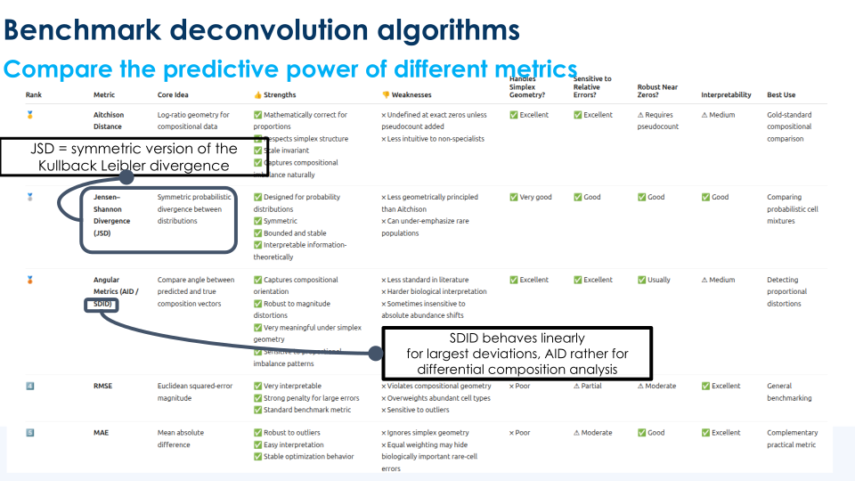
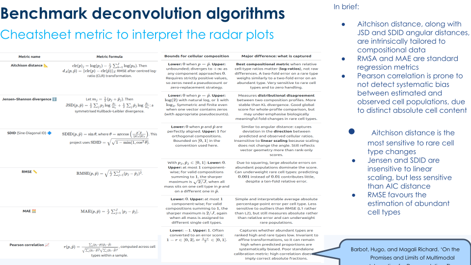
Every distance below is an error unless noted (F1, Pearson, coverage): 0 is ideal whenever a canonical bound exists. Figure 9 shows how L_1, L_2, L_{\infty}, Aitchison, and angular balls sit on the simplex; Note 13 reads that geometry.

(a) Simplex geometry of L_1, L_2, L_{\infty}, Aitchison, and angular discrepancies between \boldsymbol{p}^{\star} and \hat{\boldsymbol{p}}.

(b) How those distances behave near the barycentre versus near a vertex of the simplex.

Figure 9: Compositional error metrics for \boldsymbol{p} on \Delta^{J-1}.

Note 13: Euclidean versus log-ratio geometry on the simplex

Compositions live on \Delta^{J-1}, not in \mathbb{R}^{J} (Aitchison 1982). The same Euclidean vector \boldsymbol{e}=\hat{\boldsymbol{p}}-\boldsymbol{p}^{\star} therefore has a different meaning at the barycentre than near a vertex (Figure 9 (b)).

• RMSE / MAE / MaxAE treat a 0.05 miss on a type with p_j=0.50 like a 0.05 miss on a type with p_j=0.01. Abundant types dominate. On the simplex the sharp bounds are \|\boldsymbol{e}\|_1\le 2, \|\boldsymbol{e}\|_2\le\sqrt{2}, \|\boldsymbol{e}\|_\infty\le 1 (all mass on one type in \boldsymbol{p}^{\star} and on a different type in \hat{\boldsymbol{p}}), not the coordinate-wise bound of one.
• Total variation d_{\mathrm{TV}}=\tfrac12\|\boldsymbol{e}\|_1 is that L_1 geometry already scaled to [0,1]. It is the package default global absolute error (tv); MAE is \|\boldsymbol{e}\|_1/J=2\,d_{\mathrm{TV}}/J.
• Aitchison / CLR scores relative (log-ratio) error, so a two-fold miss on a rare type weighs like a two-fold miss on an abundant type. The distance is unbounded and undefined at exact zeros without a replacement. DeCovarT does not return it from compute_benchmark_metrics() (Table 9).
• Jensen–Shannon is a bounded, symmetric disagreement of two discrete distributions (Lin 1991). The associated distance \sqrt{\mathrm{JSD}/\log 2} is a metric (Endres and Schindelin 2003). It is gentler than Aitchison on rare types and finite with zeros after a standard convention 0\log 0=0. It is likewise not a primary package column.
• Angular / SDID ignore amplitude along a ray. On the simplex the total mass is already one, so they mainly capture whether the two compositions point the same way (including near-orthogonal spills onto the wrong vertex).

Composition and regression scores

Global scores are computed per bulk column. Cell-type Pearson, F1, and false-positive mass are aggregated across samples for each type; they are not the within-sample correlation of the length-J vectors, which is unstable for small J.

Table 8: Kept composition and regression scores from compute_benchmark_metrics() (R/utils-metrics.R).

Metric	Formula	Bounds	Captures	Pros_cons
Absolute error	Absolute error	Absolute error	Absolute error	Absolute error
Total variation / nMAE (tv)	\(d_{\mathrm{TV}}=\tfrac12\|e\|_1\)	\([0,1]\) (equals \(\|e\|_1/2\))	Mean absolute percentage-point error, simplex-normalised	Interpretable; \(J\)-free. Underweights relative rare-type error.
MaxAE (maxae)	\(\max_j |e_j|\)	\([0,1]\)	Worst single cell-type miss	Safety diagnostic. Ignores all non-maximum errors.
Quadratic error	Quadratic error	Quadratic error	Quadratic error	Quadratic error
RMSE (rmse)	\(\sqrt{J^{-1}\sum_j e_j^2}\)	\([0,\sqrt{2/J}]\); \(L_2/\sqrt{2}\) is \(J\)-free	Large absolute misses (abundant types dominate)	Familiar \(L_2\) penalty. Dominated by abundant types.
Angular	Angular	Angular	Angular	Angular
Normalised angular distance (angular)	\(d_\theta=(2/\pi)\arccos(p^{\top}\hat p/(\|p\|_2\|\hat p\|_2))\)	\([0,1]\)	Direction between the two compositions	Bounded metric. Partly redundant once \(\sum p_j=1\).
SDID (sdid)	\(\sqrt{\sin\theta}=(1-\cos^{2}\theta)^{1/4}\)	\([0,1]\)	HADACA angular companion of \(d_\theta\)	Continuity with HADACA3. Less standard than \(d_\theta\).
Association (cell type)	Association (cell type)	Association (cell type)	Association (cell type)	Association (cell type)
Pearson \(r\) (pearson)	\(\mathrm{cor}(\{p_{ij}\}_i,\{\hat p_{ij}\}_i)\)	\([-1,1]\); error \((1-r)/2\in[0,1]\)	Ranking of samples for one type, not calibration	Detects orderings across samples. High \(r\) can hide bias.
Boundary / spillover	Boundary / spillover	Boundary / spillover	Boundary / spillover	Boundary / spillover
Presence F1 (presence_f1)	\(F_1=2PR/(P+R)\) at threshold \(\varepsilon=10^{-4}\)	\([0,1]\) (\(1\) best)	Recovery of present versus absent types	Rare/absent types visible. Threshold-sensitive.
False-positive mass	\(N^{-1}\sum_i\sum_{j:p_{ij}\le\varepsilon}\hat p_{ij}\)	\([0,1]\)	Mass spilled onto truly absent types	Direct spillover mass. Needs a true zero set.
Reconstitution (no \(p^{\star}\))	Reconstitution (no \(p^{\star}\))	Reconstitution (no \(p^{\star}\))	Reconstitution (no \(p^{\star}\))	Reconstitution (no \(p^{\star}\))
Reconstitution MAE / Pearson	\(\|y-\mu\hat p\|_1/G\); \(\mathrm{cor}(y,\mu\hat p)\)	MAE on \(y\): data-scale; \(r\in[-1,1]\)	How well \(\hat p\) rebuilds the bulk when \(p^{\star}\) is unknown	Works without \(p^{\star}\). Can look good with a wrong \(\hat p\).

Table 9: Related composition scores that are not primary compute_benchmark_metrics() columns.

Metric	Formula	Bounds	Captures	Why_not
Absolute error	Absolute error	Absolute error	Absolute error	Absolute error
MAE (helper .mae() only)	\(J^{-1}\|e\|_1=2\,d_{\mathrm{TV}}/J\)	\([0,2/J]\); \(J\)-free form is \(d_{\mathrm{TV}}\)	Same \(L_1\) information as TV at fixed \(J\)	Report tv instead (already \([0,1]\)).
Log-ratio	Log-ratio	Log-ratio	Log-ratio	Log-ratio
Aitchison distance	\(\|\mathrm{clr}(p)-\mathrm{clr}(\hat p)\|_2\)	\([0,\infty)\); undefined at structural zeros	Relative (fold-change) error, rare types included	Zero replacement dominates; no canonical \([0,1]\) bound.
Information	Information	Information	Information	Information
Jensen–Shannon divergence / distance	\(\tfrac12\mathrm{KL}(p\|m)+\tfrac12\mathrm{KL}(\hat p\|m)\), \(m=(p+\hat p)/2\)	\([0,\log 2]\) (nats); distance \(\sqrt{\mathrm{JSD}/\log 2}\in[0,1]\)	Symmetric distributional disagreement	Not implemented in R/utils-metrics.R.
Probability geometry	Probability geometry	Probability geometry	Probability geometry	Probability geometry
Hellinger distance of compositions	\(2^{-1/2}\|\sqrt{p}-\sqrt{\hat p}\|_2\)	\([0,1]\)	Hellinger geometry of \(\sqrt{p}\); zeros allowed	Monotone with \(L_2\) on square-root compositions; not wired.
Association	Association	Association	Association	Association
Sample-wise Pearson of the \(J\)-vector	\(\mathrm{cor}_j(p,\hat p)\) within one sample	\([-1,1]\)	Within-sample ranking of types	Unstable for small \(J\); high \(r\) hides calibration error.
Spearman \(\rho_S\)	rank correlation across samples	\([-1,1]\)	Monotone ranking, magnitudes discarded	Ignores absolute fractions.
Hierarchical	Hierarchical	Hierarchical	Hierarchical	Hierarchical
Hierarchical relative RMSE (hrRMSE)	RMSE scaled by nested biological variance	scale depends on the ontology	Error relative to a cell-type hierarchy	Needs a cell-type ontology [@baWhenLessNot2026]; @fig-hrrmse.

Figure 10: Hierarchical relative RMSE (hrRMSE) used when some reference types are missing: residual error is scaled by the biological variance of \boldsymbol{p}^{\star} rather than by raw proportion units (Ba et al. 2026).

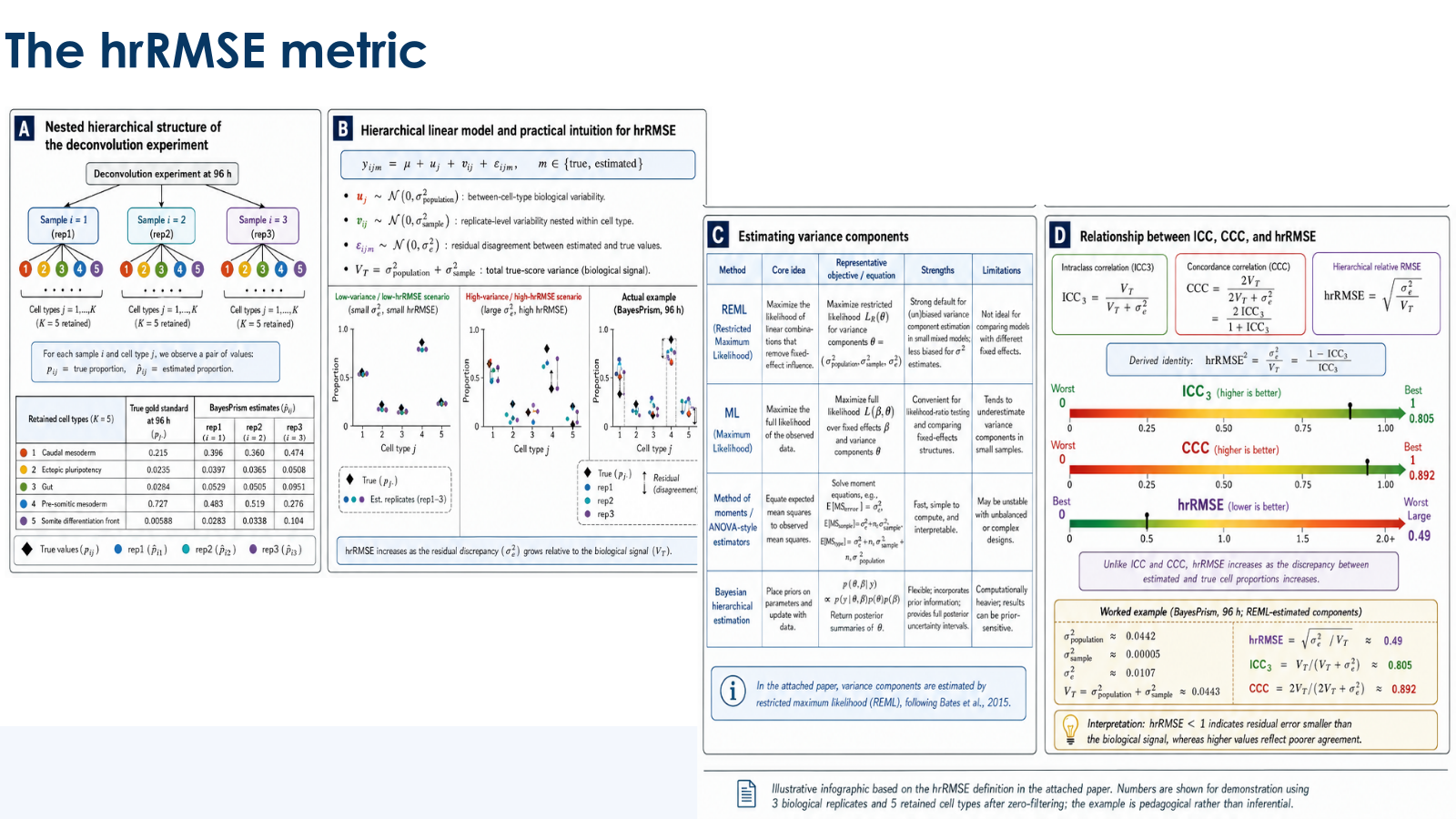
Note 14: Angular distance versus SDID

Both scores are strictly increasing functions of the same angle \theta=\arccos(p^{\mathsf{T}}\hat p/(\|p\|_2\|\hat p\|_2)). The normalised angular distance d_\theta=2\theta/\pi is a metric on [0,1]. SDID is \sqrt{\sin\theta} (the HADACA convention implemented in .sdid()). They rank methods identically; report one in the headline panel and keep the other for continuity with HADACA3 (Barbot and Richard 2026).

Note 15: Simplex bounds for L_p errors

Because \boldsymbol{p} and \hat{\boldsymbol{p}} both sum to one and are non-negative, \boldsymbol{e} is orthogonal to \mathbf{1} and cannot put unit mass on two opposite vertices at once without taking it from the other. Hence \|\boldsymbol{e}\|_1\le 2, \|\boldsymbol{e}\|_2\le\sqrt{2}, and \|\boldsymbol{e}\|_\infty\le 1, with equality when all mass sits on one type in \boldsymbol{p} and on a different type in \hat{\boldsymbol{p}}. Normalised MAE is total variation: J\,\mathrm{MAE}/2=d_{\mathrm{TV}}. Raw RMSE still depends on J; divide by \sqrt{2/J} (equivalently \|\boldsymbol{e}\|_2/\sqrt{2}) if a dimension-free L_2 score is needed.

Monte Carlo (ADEMP) summaries

These describe the estimator as a repeated-sampling procedure, not the distance between one \hat{\boldsymbol{p}} and one \boldsymbol{p}^{\star}. Each row of monte_carlo is one cell type. Coverage intervals around the rate \hat\pi are derived in Note 20.

Table 10: Kept Monte Carlo / ADEMP summaries (monte_carlo block and coverage_mc_interval()).

Metric	Formula	Bounds	Captures	Pros_cons
Point estimation	Point estimation	Point estimation	Point estimation	Point estimation
Bias (bias)	\(B^{-1}\sum_b \hat p_{jb}-p_j\)	\([-1,1]\); \(|\mathrm{bias}|\in[0,1]\)	Signed systematic error per cell type	Direction of miscalibration. Joint biases can cancel in a global score.
Monte Carlo RMSE (rmse)	\(\sqrt{B^{-1}\sum_b(\hat p_{jb}-p_j)^2}\)	\([0,1]\) on a \([0,1]\) coordinate	Bias and variance on the composition scale	Single accuracy number. Mixes bias and variance (report both).
Sampling precision	Sampling precision	Sampling precision	Sampling precision	Sampling precision
Empirical SD (empirical_sd)	\(\sqrt{(B-1)^{-1}\sum_b(\hat p_{jb}-\bar p_j)^2}\)	population SD \(\le 1/2\) on \([0,1]\)	Monte Carlo precision of \(\hat p_j\)	Direct sampling SD. Sample SD can slightly exceed \(1/2\).
Reported uncertainty	Reported uncertainty	Reported uncertainty	Reported uncertainty	Reported uncertainty
Mean model SE (mean_model_se)	\(B^{-1}\sum_b \widehat{\mathrm{SE}}_{jb}\)	no guaranteed finite bound (Wald SE)	Mean claimed Wald (or supplied) standard error	Tests the uncertainty estimate itself. Poor near the boundary.
SE calibration	SE calibration	SE calibration	SE calibration	SE calibration
SE / SD ratio (se_sd_ratio)	\(\overline{\widehat{\mathrm{SE}}}_j / \mathrm{SD}(\hat p_j)\)	\([0,\infty)\); \(1\) is calibrated	Under- versus over-stated uncertainty	Direct diagnosis. Unstable when empirical SD is tiny.
Combined accuracy	Combined accuracy	Combined accuracy	Combined accuracy	Combined accuracy
Mean model SD (mean_model_sd)	\(\sqrt{B^{-1}\sum_b \widehat{\mathrm{SE}}_{jb}^{2}}\)	same units as empirical SD	RMS of reported SEs (compares to empirical SD)	Companion to mean SE. Not a substitute for coverage.
Interval inference	Interval inference	Interval inference	Interval inference	Interval inference
Coverage (coverage)	\(B^{-1}\sum_b \mathbf{1}\{L_{jb}\le p_j\le U_{jb}\}\)	\([0,1]\); target \(1-\alpha\), not \(1\)	Frequentist calibration of the interval for \(p_j\)	Essential inferential check. Rewards overly wide intervals if used alone.
Mean interval width	\(B^{-1}\sum_b(U_{jb}-L_{jb})\)	\([0,1]\) for simplex-clipped intervals	Precision of the interval, given coverage	Separates useful from vacuous coverage. Smaller is not better unless coverage holds.
MCSE of coverage (mcse_coverage)	\(\sqrt{\hat\pi(1-\hat\pi)/B}\)	\([0,1/\sqrt{4B}]\)	Simulation error of the coverage rate	Binomial MCSE. Wald form of the rate; interval for \(\hat\pi\) uses Wilson.

Table 11: ADEMP-adjacent diagnostics that are not default columns.

Metric	Formula	Bounds	Captures	Why_not
Boundary inference	Boundary inference	Boundary inference	Boundary inference	Boundary inference
Endpoint-at-zero / active-set F1	\(B^{-1}\sum_b 1\{\min_j\hat p_{jb}\le\tau\}\)	\([0,1]\)	How often estimates sit on a face	Scenario-specific; presence F1 already summarises support.
Testing	Testing	Testing	Testing	Testing
Type-I error	rejection rate under \(H_0\)	\([0,1]\); target \(\alpha\)	False detections of a cell type	Requires an explicit \(H_0\) grid (out of ADEMP scope here).
Power	rejection rate under a designed alternative	\([0,1]\)	Ability to detect a designed shift	Requires a designed alternative (out of scope).
Landscape	Landscape	Landscape	Landscape	Landscape
Multistart likelihood spread	\(\max_s\ell_s-\min_s\ell_s\) among converged starts	\([0,\infty)\)	Distinct basins of the likelihood	Needs multi-start logging (multistart_decovart()), not default.
Constraints	Constraints	Constraints	Constraints	Constraints
Simplex violation	distance of \(\hat p\) to \(\Delta^{J-1}\) before repair	\([0,\infty)\)	Constraint fidelity of the raw solver return	Solvers already repair onto the simplex (repair_simplex()).
Linear algebra	Linear algebra	Linear algebra	Linear algebra	Linear algebra
Cholesky fill-in / sparse timings	nnz$(L)$ or seconds per factorisation	non-negative	Cost of \(\Sigma(p)^{-1}\) at the chosen structure	Appendix S2; declare the covariance structure.

Note 16: Monte Carlo standard error of coverage

Coverage is a mean of i.i.d. Bernoulli indicators I_b=\mathbf{1}\{p_j\in\mathrm{CI}_{jb}\}. With B independent simulated datasets,

\widehat{\mathrm{MCSE}} = \sqrt{\hat\pi(1-\hat\pi)/B}.

The denominator is B, not B times an inner bootstrap size: bootstrap draws belong to the interval algorithm, not to the outer simulation. At true 95% coverage, B=1000 gives \mathrm{MCSE}\approx 0.0069. The package stores mcse_coverage on the monte_carlo table. For a generic mean \widehat T=B^{-1}\sum_b T_b, use \widehat{\mathrm{MCSE}}(\widehat T)=s_T/\sqrt{B} (.mcse_mean()).

Execution and optimisation

Numerical convergence is whether the solver returned a finite simplex vector. Theoretical convergence asks whether \ell(\hat{\boldsymbol{p}}) is within 10^{-3} of \ell(\boldsymbol{p}^{\star}) (the generating value, a proxy for the expected global maximum in a well-specified Monte Carlo). The default stationarity diagnostic stored on optimisation$kkt_residual is the simplex projected-score residual .kkt_residual() (Note 17), not the raw ambient gradient and not the ILR score from boundary_diagnostics().

Elapsed time is the per-sample proc.time() elapsed inside each worker. Memory is process PSS from ps (RSS if PSS is unavailable). Both are stored as full per-sample vectors in optimisation.

Table 12: Kept optimisation and runtime scores (optimisation block).

Metric	Formula	Bounds	Captures	Pros_cons
Convergence	Convergence	Convergence	Convergence	Convergence
Numerical convergence (numerical_converged)	finite simplex return; no solver error	rate in \([0,1]\) (ideal \(1\))	Operational reliability of the solver return	Mandatory runtime check. A finite \(p\) need not be stationary.
Theoretical convergence (theoretical_converged)	\(\ell(p^{\star})-\ell(\hat p)\le 10^{-3}\)	rate in \([0,1]\) (ideal \(1\))	Whether \(\hat p\) attains (nearly) the generating likelihood	Detects poor modes when \(p^{\star}\) is known. Proxy, not global uniqueness.
KKT / projected-score residual (kkt_residual)	\(\|\Pi_\Delta(\hat p+\nabla_p\ell)-\hat p\|_2\)	\([0,\infty)\); \(0\) is first-order stationary	Simplex KKT first-order residual, including faces	Boundary-aware; solver-independent. Small residual is not global optimality.
Likelihood	Likelihood	Likelihood	Likelihood	Likelihood
Log-likelihood regret (loglik_regret)	\(\ell(p^{\star})-\ell(\hat p)\)	\((-\infty,\infty)\); \(0\) matches \(\ell(p^{\star})\)	Likelihood gap to the data-generating composition	Scale-free comparison of modes. Requires \(p^{\star}\) and \(\Sigma\).
Runtime	Runtime	Runtime	Runtime	Runtime
Elapsed time (elapsed_sec)	worker elapsed seconds for one column of \(Y\)	\([0,\infty)\)	Per-sample computational cost	Direct utility. Hardware-dependent; report median / IQR.
Peak memory (memory_bytes)	ps::ps_memory_full_info()$pss in the worker	\([0,\infty)\) bytes	Per-sample memory footprint (PSS, not summed RSS)	Avoids double-counting shared pages. Still machine-dependent.

Table 13: ILR score and Hessian extrema are now stored on optimisation; wall time of the whole job is not.

Metric	Formula	Bounds	Captures	Why_not
ILR geometry	ILR geometry	ILR geometry	ILR geometry	ILR geometry
ILR score norm (score_norm)	\(\|\nabla_{z}\tilde\ell(\hat z)\|_2=\|J_{\psi}^{\top}\nabla_p\ell\|_2\)	\([0,\infty)\); \(0\) is interior stationarity	Unconstrained first-order residual in ILR coordinates	Interior equivalent of KKT, but the Jacobian degenerates on faces (@nte-kkt-ilr-hessian).
Curvature	Curvature	Curvature	Curvature	Curvature
Tangent / ILR \(\lambda_{\min},\lambda_{\max}(H)\) (min_eigenvalue, max_eigenvalue)	\(\lambda_{\min}(H_z),\lambda_{\max}(H_z)\) of hessian_loglik_constrained()	unbounded; both \(<0\) at a local maximum	Local max versus saddle in the ILR chart	Local only; local_maximum is a flag on boundary_diagnostics(), not a column of optimisation.
Speed	Speed	Speed	Speed	Speed
End-to-end wall time of the parallel job	clock around deconvolute_ratios()	\([0,\infty)\)	Throughput of the whole Monte Carlo job	Confounds scheduling with per-sample cost.
Memory	Memory	Memory	Memory	Memory
Sum of worker RSS	sum of per-worker RSS	\([0,\infty)\)	Naive memory sum under fork	Double-counts copy-on-write pages.

Note 17: Interior ILR stationarity, projected KKT residual, and Hessian curvature

Three numbers are easy to confuse. They answer different questions, and only the second is the default kkt_residual column.

Ambient score. DeCovarT differentiates \ell(\boldsymbol{p}) with \boldsymbol{p} treated as free coordinates (gradient_loglik_unconstrained()). On the simplex that vector need not vanish at a maximum. An interior stationary point satisfies g_1=\cdots=g_J=\lambda: every feasible direction \boldsymbol{d} has \mathbf{1}^{\top}\boldsymbol{d}=0, so \boldsymbol{g}^{\top}\boldsymbol{d}=0 as soon as \boldsymbol{g} is constant. Reporting \|\nabla_p\ell\|_2 is therefore a bad convergence diagnostic.

Interior ILR score. Native DeCovarT solvers optimise in isometric log-ratio coordinates z=\mathrm{ilr}(\boldsymbol{p}) (Helmert chart). The unconstrained first-order condition is \nabla_z\tilde\ell(\hat z)=0, implemented as score_norm in boundary_diagnostics(): \nabla_z\tilde\ell=J_{\psi}^{\top}\nabla_p\ell. For p_j>0, J_{\psi}^{\top}g=0 if and only if P_T g=0 with P_T=I-J^{-1}\mathbf{1}\mathbf{1}^{\top}, because the columns of J_{\psi} span the simplex tangent space. The norms are not the same: \|J_{\psi}^{\top}g\|_2\neq\|P_T g\|_2 in general. Near a face, p_j\to 0 and \|z\|\to\infty; entries of J_{\psi} contain factors of p_j, so \|\nabla_z\tilde\ell\| can look small because the chart is flattening rather than because the ambient KKT violation is small. boundary_diagnostics() therefore skips score_norm when \min_j\hat p_j is below boundary_tol.

Projected-score / KKT residual (headline). For maximisation, R_{\alpha}(\boldsymbol{p}) = \alpha^{-1}\bigl( \Pi_{\Delta}(\boldsymbol{p}+\alpha\nabla_p\ell) -\boldsymbol{p} \bigr), with Euclidean projection \Pi_{\Delta} onto the simplex (.project_simplex()) and default \alpha=1. Then \texttt{kkt\_residual}=\|R_{\alpha}(\hat{\boldsymbol{p}})\|_2. This vanishes if and only if a first-order feasible step does not move the iterate, including when some p_j=0 (KKT: g_j=\lambda on the support, g_j\le\lambda on inactive types). That is the quantity stored by deconvolute_ratios().

Hessian / curvature. First-order stationarity does not imply a local maximum. boundary_diagnostics() reports both \lambda_{\min}(H_z) and \lambda_{\max}(H_z) of hessian_loglik_constrained() and sets local_maximum when the ILR score is below score_tol and the Hessian is negative definite (both eigenvalues strictly negative). A small KKT residual with \lambda_{\min}<0<\lambda_{\max} is a saddle. None of these diagnostics implies a unique global mode; the DeCovarT likelihood for one bulk sample is not concave in general (MLE properties).

Note 18: Which metric to report

Use TV, RMSE, MaxAE, and (optionally) angular distance / SDID as the global panel. Add cell-type Pearson and presence F1 / false-positive mass when rare or absent types matter (Sturm et al. 2019; Avila Cobos et al. 2020). Report ADEMP bias, empirical SD, SE/SD, coverage (with MCSE and a Wilson interval on the rate), and mean width whenever intervals exist. Quote median and IQR of elapsed time and PSS from the optimisation table rather than a single end-to-end clock. Pair kkt_residual with numerical_converged and theoretical_converged; the three stacked-bar outcomes in Figure 11 partition every replicate. Quote score_norm / local_maximum only for interior ILR fits, and report both \lambda_{\min}(H_z) and \lambda_{\max}(H_z) so a saddle (\lambda_{\min}<0<\lambda_{\max}) is not mistaken for a maximum.

Monte Carlo solver outcomes as an Euler diagram: numerical failure is nested in theoretical failure; theoretical success is disjoint.

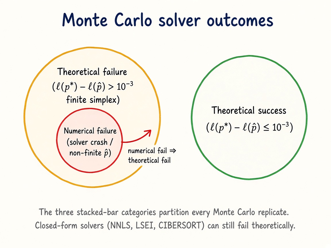
Figure 11: Euler diagram of the three ADEMP solver outcomes. Numerical failure (solver crash or a non-finite simplex) implies theoretical failure, so the red disc sits inside the amber set. Theoretical success is the disjoint green disc. Stacked bars in output/fig02/performance_visualisations/convergence_stacked.pdf and the fig03 counterpart count these three categories on the same corner layout as the Wald forest.

Warning 19: Why some raincloud panels look empty

Two distinct mechanisms produced blank \hat p rainclouds on the fig02 book.

• Legend overlay. The four correlation corners are arranged as a 2\times 2. rho = (-0.8, 0.8) is the bottom-right facet. An inset cowplot legend at (x,y)=(0.68,0.08) sat on top of that panel. The legend now sits to the right of the facets (cowplot::get_legend()).
• Vertex pile-up. On highly unbalanced compositions (rho = (0, 0), small CLD, homoscedastic), many solvers pin a rare type at 0 and the abundant type at 1. A bounded kernel density on [0,1] with almost no unique values emits an empty slab. The raincloud helper now overlays Monte Carlo dots whenever a group has two or fewer distinct estimates.

Neither blank is a missing numerical_converged flag. Check the stacked-bar book before interpreting an empty density as a solver crash.

Zoom on the coverage rate, and derivation of the intervals

Wilson is the default interval around the estimated coverage rate \hat\pi=X/N, not the interval for \hat p_j (Wilson 1927). The interval for p_j on an interior composition is the ILR delta-method Wald interval from vcov_ilr_delta() / confint.decovart_fit(): expected Fisher information of the Gaussian convolution, pulled back through the isometric log-ratio chart — not the observed Hessian of a Newton step, and not an ALR chart. Wald and Agresti–Coull (Agresti and Coull 1998) are available through coverage_interval for the binomial rate. Bias-eliminated coverage (covering \bar{\hat\theta} rather than \theta) is not implemented; report ordinary coverage and bias side by side instead. Note 20 summarises exact, asymptotic, and optimisation-based constructions for that binomial rate.

Note 20: Intervals for a binomial coverage rate

The Monte Carlo coverage rate \hat\pi=X/N is a binomial proportion on the unit interval. Interval construction for that rate is not a confidence interval for the cell-type vector \boldsymbol{p}. Three strategies are in common use (Agresti and Coull 1998; Konietschke and Brunner 2026).

• Asymptotic (Wald, Wilson, Agresti–Coull). The Wald interval is \hat\pi\pm z\sqrt{\hat\pi(1-\hat\pi)/N}. Near 0 or 1 the estimated standard error collapses and the interval can leave [0,1] (the classic edge-case failure). Wald is a poor default for coverage rates. The Wilson score interval (Wilson 1927) is the package default: it is widely used, remains inside (0,1) for interior \hat\pi, and is more stable near the boundary. Agresti–Coull is the optional adjusted-Wald form already exposed by coverage_interval.
• Exact (test inversion). Clopper–Pearson-type intervals invert binomial tail probabilities and guarantee a minimum coverage of at least 1-\alpha, at the cost of systematic conservatism. Length–coverage optimal (LCO) methods change the acceptance region itself so that minimum coverage is guaranteed while average length is reduced; they remain conservative by construction.
• Optimisation-based calibration. Because the binomial sampling distribution is discrete, no interval attains exact nominal coverage uniformly in \pi\in(0,1). Numerical level adjustment treats the critical value or tail probability as a scalar \gamma and retunes a fixed analytical form. Konietschke and Brunner (2026) minimise a risk functional of the exact coverage curve (for example mean squared deviation from 1-\alpha, or absolute deviation of average coverage) for Wilson, Agresti–Coull, logit, or Clopper–Pearson formulae without rewriting those formulae. The method is aimed at small N.

DeCovarT does not implement tuned or LCO intervals. Independent Monte Carlo replicates N can be increased arbitrarily, so the small-sample discreteness problem that motivates optimisation-based tuning is not the operating regime. Report ordinary Wilson (or Agresti–Coull) intervals on \hat\pi, together with mcse_coverage and bias, rather than a small-sample recalibration of \gamma.

Asymptotic normality of \hat{\boldsymbol{p}}

Batardière, Chiquet and Mariadassou inspect studentised variational estimates against N(0,1) with Q-Q plots and a one-sample Kolmogorov–Smirnov test (Batardière et al. 2024). The same two displays are useful here, with one modelling caveat: DeCovarT’s \hat{\boldsymbol{p}} is a constrained maximum-likelihood estimator of the Gaussian convolution, so first-order MLE theory applies on the interior of the simplex. Their sandwich correction is for a variational estimator of a Poisson-log-normal latent-variable model, which is not itself an MLE and does not inherit those consistency guarantees (Westling and McCormick 2019). Do not treat the two studentisations as interchangeable.

Q-Q plots of the whitened ILR coordinates W=I_{\boldsymbol{z}}(p^{\star})^{1/2}(\hat{\boldsymbol{z}}-\boldsymbol{z}^{\star}) use a single tail-sensitive qqplotr band (Aldor-Noiman et al. 2013) calibrated to the theoretical N(0,1) law (identity = TRUE, mu = 0, sigma = 1; not detrended). Colour and fill distinguish L-BFGS, Marquardt–Levenberg and Newton–Raphson; gradient and simulated annealing are omitted. A companion PDF Q-Q-plots the joint Mahalanobis statistic D^{2}=W^{\mathsf{T}}W against \chi^{2}_{J-1}. The KS lollipops report one p-value per scenario \times solver: below 0.05 we reject normality at the conventional 5% level. qqplotr needs system libfftw3. The books are output/fig02/performance_visualisations/qq_normal.pdf, qq_chi2.pdf and ks_normal.pdf (and the fig03 counterparts).

Figure 12: Q-Q plots: points hug the diagonal when the normal assumption holds, and curve away when it does not. Normal: points on the line. Heavy tails: S-curve, ends flare. Right-skewed: concave-up bend. Light tails: flatter S-shape.

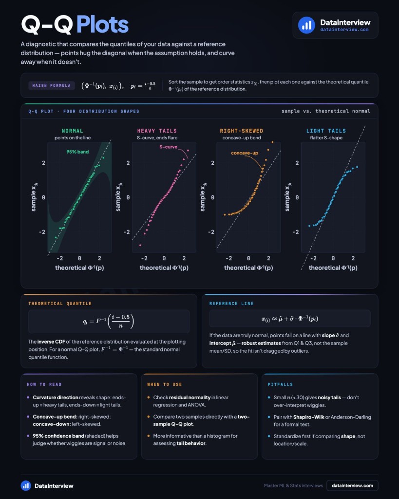
Hazen plotting positions p_i=(i-0.5)/n against \Phi^{-1}(p_i), after Aldor-Noiman et al. and the DataInterview explainer. Curvature direction diagnoses tail weight and skew; a 95% band helps separate signal from Monte Carlo wiggle.

Warning 21: Do not promote a Kolmogorov–Smirnov p-value to a verdict

The KS lollipops are a companion to the Q-Q books, not a substitute.

• The p-value fallacy. A small p does not measure the size of the departure from normality, and a large p does not prove the normal approximation (Goodman 1999). Increasing the Monte Carlo size N will reject any fixed alternative, however tiny.
• Compare magnitudes, not stars. Olszewski’s argument against two-sample t-tests of arithmetic means applies equally here: plot the distributions, and prefer estimation over ritualised p-values. Rainclouds already show bias, variance, skew and boundary pile-up; the Q-Q plot shows tail behaviour. The KS p adds a single scalar that conflates those features.

Note 22: No p-value for the coverage rate

Coverage of a Wald interval is the Monte Carlo mean of the indicator I\{\theta_0\in\mathrm{CI}_m\}, not a test of |(\hat\theta-\bar{\hat\theta})/s|<1.96. That second quantity studentises against the Monte Carlo mean rather than against \theta_0, and the unit-simplex constraint already invalidates a symmetric \pm 1.96\,\widehat{\mathrm{SE}} statement near a face. Reporting a p-value for the coverage rate would duplicate the indicator without adding a new estimand. Report \hat\pi, its Wilson interval, mcse_coverage, and bias side by side instead.

Conclusions

A reproducible synthetic study should keep three design layers separate, then score both the reference geometry and the mixture composition:

1. Mean signatures. Build \boldsymbol{\mu} with generate_mean_signature_matrix(): hold mean_scale s fixed and dial the Gram R (target_cosine or target_gram). Report the realised pairwise cosine (it equals R up to rounding), Euclidean separation, and optionally \kappa_2(\boldsymbol{\mu}).
2. Precision graphs. Draw an undirected skeleton (scale_free, stochastic_block_model, or small_world), assign i.i.d. signed weights (prop_inhibitory), and complete \Omega\succ 0 by the uniform spectral shift. Report \kappa(\Omega) and the partial-correlation sign mix.
3. Cellular compositions. Choose \boldsymbol{p} on a Shannon grid from uniform (H^{\star}=1) to near-pure (H^{\star}\approx 0), matching the SimBu fraction vocabulary when comparing to pseudo-bulk tools (Figure 7).

See Note 23 for a compact factorial checklist.

Important 23: Recommended benchmark specification

Use one pipeline for a given topology of a given cell type’s covariance structure (Eq. 16, Figure 4):

\text{topology} \rightarrow \text{signed weights} \rightarrow \text{SPD precision} \rightarrow \text{mean design} \rightarrow \text{latent Gaussian} \rightarrow \text{observation model} \tag{16}

Prefer: - uniform spectral shift (Eq. 12) or partial-correlation scaling (Eq. 11) when support and signs are exact; G-Wishart when support and signs are approximate. - composition grid from uniform (H^{\star}=1) to near-pure (H^{\star}\approx 0), matching the SimBu fraction vocabulary when comparing to pseudo-bulk tools (Figure 7). - add the mean layer independently of graph generation.

Note 24: Execution: no nested parallelism, furrr, L’Ecuyer streams

Sample-level workers live only in deconvolute_ratios(). .map_samples() calls furrr::furrr_options(seed = TRUE), which is the R \ge 4.1 / future implementation of independent L’Ecuyer-CMRG streams per worker (Morris et al. 2019). run_simulation_benchmark() evaluates scenario rows sequentially, so streams are never nested. Do not offset a shared seed by the sample index (set.seed(seed + i)). For an explicit cluster script, set RNGkind("L'Ecuyer-CMRG") once and advance with parallel::nextRNGStream, or keep furrr seed = TRUE.

That furrr path is the default for long jobs and for reproducible benchmarks. mirai (persistent daemons, dynamic dispatch) is reserved for APIs that need a fast interactive response, not for the published Monte Carlo protocol.

Perspectives on high-dimensional or more biologically realistic designs

Beyond the families in Table 1:

• Degree-prescribed / configuration graphs separate degree heterogeneity from preferential-attachment mechanisms.
• Spatial / geometric graphs suit spatial transcriptomics or chromatin neighbourhoods.
• Differential networks:
  • Start from a shared base G_0
  • Control the differential shift \Omega_k=\Omega_0+\Delta_k
  • Ensure the SPD step
  • Alternatively, vary the support, weight, and sign separately (Federico et al. 2023; Wu and Luo 2022).
• Other distributions, using the GGM layer as a parameter:
  • Latent-variable GGMs — sparse \Omega_S plus low-rank confounding Bf_i.
  • Nonparanormal / Gaussian-copula margins on a latent Gaussian graph.
  • Poisson–log-normal / compositional observation layers on latent log-abundances (Chiquet et al. 2018).
  • Zero-inflated mixture GGMs with cell-type-specific (\mu_k,\Omega_k) and expression-dependent dropout (Wu and Luo 2022).

Simulation reporting: ADEMP and Nature Methods

This section is a reporting checklist for DeCovarT simulation studies, not a new experiment. It maps package outputs onto the ADEMP structure of Morris, White and Crowther (Morris et al. 2019) and onto the Nature Methods requirements for data, code and statistical reporting (reporting standards).

There is no composite global score. Global composition distances, cell-type Pearson / F1, and Monte Carlo operating characteristics answer different questions and must stay in separate tables.

The estimand is the composition \boldsymbol{p} on the simplex. The data-generating mechanism is the Gaussian convolution \boldsymbol{y}\mid(\boldsymbol{\zeta},\boldsymbol{p})\sim \mathcal{N}_{G}(\boldsymbol{\mu}\boldsymbol{p},\sum_j p_j^2\boldsymbol{\Sigma}_j). Methods are the solvers passed to deconvolute_ratios().

Table 14: ADEMP performance measures implemented in compute_benchmark_metrics() and coverage_mc_interval().

ADEMP	Package
Aims	Compare solvers on a known convolution
Data-generating mechanism	simulate_bulk_mixture() + describe_simulation_scenario()
Estimand	p (simplex); cell-type and global scores kept separate
Methods	deconvolute_ratios() / fit_decovart()
Bias	bias
Empirical SE	empirical_sd
Model SE	mean_model_se (and mean_model_sd)
Relative error in SE	se_sd_ratio
RMSE	rmse (cell type) and regression$global$rmse
Coverage	coverage with Wilson interval by default
Mean interval width	mean_interval_width
Monte Carlo SE of coverage	mcse_coverage
Convergence	numerical_converged, theoretical_converged, kkt_residual
Type I / power	Not a primary target (composition estimation, not a null test)

Visualisation plots:

• plot_mc_raincloud() shows the sampling distribution of \hat p_j-p_j^{\star}; inner / outer bars are empirical Monte Carlo quantiles, not a CI for p (Allen et al. 2019).
• plot_mc_forest() is the ADEMP ranking companion (Wilson whiskers on the coverage rate).
• plot_algorithm_similarity() is behavioural correlation of \hat{\boldsymbol{p}}, not numerical agreement.
• plot_mc_metric_dots() facets by metric with a single min–max colour scale.

Nature Methods reporting

Nature Methods requires a reporting summary, a data-availability statement, and promptly available code and protocols. The mapping below is the package counterpart of that editorial checklist.

Table 15: Nature Methods reporting items covered by the simulation API.

Requirement	Where it lives in DeCovarT
Data-generating mechanism fully specified	theta_true (p, mu, sigma) plus descriptors and call
Estimand and metrics pre-declared	This table; compute_benchmark_metrics() blocks
Software versions	sessioninfo::session_info() in analysis scripts
Random-number streams	furrr_options(seed = TRUE): L’Ecuyer-CMRG per worker (Note 24)
Code availability	GitHub repository; package functions, not one-off scripts
No undisclosed composite score	Global and cell-type tables remain separate
Sample size / Monte Carlo error	n and mcse_coverage (and Wilson bounds)

NeurIPS code completeness

The ML Code Completeness Checklist used at NeurIPS is five items.

Table 16: NeurIPS / Papers with Code completeness mapped onto the package.

Checklist item	Where it lives
Specification of dependencies	DESCRIPTION (Imports / Suggests with versions)
Fitting (“training”) code	fit_decovart(), deconvolute_ratios()
Evaluation code	compute_benchmark_metrics(), run_simulation_benchmark()
Pre-trained models	Not applicable: DeCovarT is an estimator, not a stored neural net. Toy convolution fixtures live in inst/extdata/
README table of results plus commands	README / vignette chunks (this article; §2.1, §2.2)

rOpenSci statistical standards

rOpenSci statistical software standards are tagged in R/srr-stats-standards.R (@srrstats or @srrstatsNA) and on the exported helpers. The load-bearing blocks are:

• General / testing (G*): input checks and missing-data policy on deconvolute_ratios(); Monte Carlo tests with simulate_bulk_mixture() (G5.0, G5.5, G5.6).
• Regression (RE*): fit_decovart() return value, coef / vcov / confint, convergence, plots (RE4, RE6, RE7).
• Probability distributions (PD*): Gaussian convolution log-likelihood, score, and Hessian.

Do not add a second copy of those tags in vignettes. Runtime scaling of solvers versus (G) and (J) is documented as not applicable (G5.7, RE5.0; companion repository). ADEMP columns themselves are this section.

What is deliberately absent

• Cholesky fill-in or sparse-solver speed diagnostics (the user must declare the covariance structure; otherwise the dense Cholesky factor of \Sigma(p) is used). See Appendix S2.
• Type I error and power as default columns (the target is an estimand, not a null hypothesis). Boundary tests live in Appendix S1 and MLE properties.

References

Agresti, Alan, and Brent A. Coull. 1998. ‘Approximate Is Better Than "Exact" for Interval Estimation of Binomial Proportions’. The American Statistician 52 (2): 119–26. https://doi.org/10.2307/2685469.

Aitchison, J. 1982. ‘The Statistical Analysis of Compositional Data’. Journal of the Royal Statistical Society: Series B (Methodological) 44 (2): 139–60. https://doi.org/10.1111/j.2517-6161.1982.tb01195.x.

Aldor-Noiman, Shari, Lawrence D. Hooper, Galit Shmueli, and Ayala Cohen. 2013. ‘The Power to See: A New Graphical Test of Normality’. The American Statistician 67 (4): 249–67. https://doi.org/10.1080/00031305.2013.847865.

Aliee, Hananeh, and Fabian J. Theis. 2021. ‘AutoGeneS: Automatic Gene Selection Using Multi-Objective Optimization for RNA-seq Deconvolution’. Cell Systems 12. https://doi.org/10.1016/j.cels.2021.05.006.

Allen, Micah, Davide Poggiali, Kirstie Whitaker, Tom Rhys Marshall, Jordy van Langen, and Rogier A. Kievit. 2019. ‘Raincloud Plots: A Multi-Platform Tool for Robust Data Visualization’. Wellcome Open Research 4: 63. https://doi.org/10.12688/wellcomeopenres.15191.2.

Avila Cobos, Francisco, José Alquicira-Hernandez, Joseph Powell, Pieter Mestdagh, and Katleen De Preter. 2020. ‘Comprehensive Benchmarking of Computational Deconvolution of Transcriptomics Data’. bioRxiv, ahead of print. https://doi.org/10.1101/2020.01.10.897116.

Ba, Kalidou, Rodolphe Thiébaut, Xavier Hinaut, and Boris Hejblum. 2026. When Less Is Not More: DICEPro Mitigates the Impact of Incomplete Reference Matrices on Cellular Frequency Deconvolution. bioRxiv. https://doi.org/10.64898/2026.06.17.732876.

Barabási, Albert-László, and Réka Albert. 1999. ‘Emergence of Scaling in Random Networks’. Science 286. https://doi.org/10.1126/science.286.5439.509.

Barbot, Hugo, and Magali Richard. 2026. ‘On the Promises and Limits of Multimodal Integration for Deconvolution: The HADACA3 Benchmark’. NeurIPS.

Batardière, Bastien, Julien Chiquet, and Mahendra Mariadassou. 2024. Evaluating Parameter Uncertainty in the Poisson Lognormal Model with Corrected Variational Estimators. arXiv. https://doi.org/10.48550/arxiv.2411.08524.

Besson, Olivier, and Yuri I. Abramovich. 2013. ‘On the Fisher Information Matrix for Multivariate Elliptically Contoured Distributions’. IEEE Signal Processing Letters 20 (11): 1130–33. https://doi.org/10.1109/lsp.2013.2281914.

Broido, Anna D., and Aaron Clauset. 2019. ‘Scale-Free Networks Are Rare’. Nature Communications 10. https://doi.org/10.1038/s41467-019-08746-5.

Chiquet, Julien, Mahendra Mariadassou, and Stéphane Robin. 2018. Variational Inference for Sparse Network Reconstruction from Count Data. arXiv. https://doi.org/10.48550/arxiv.1806.03120.

Dietrich, Alexander. 2024. SimBu: Bias-Aware Simulation of Bulk RNA-Seq Data with Variable Cell-Type Composition. https://doi.org/10.18129/B9.bioc.SimBu.

Endres, D. M., and J. E. Schindelin. 2003. ‘A New Metric for Probability Distributions’. IEEE Transactions on Information Theory 49 (7): 1858–60. https://doi.org/10.1109/tit.2003.813506.

Federico, Anthony, Joseph Kern, Xaralabos Varelas, and Stefano Monti. 2023. ‘Structure Learning for Gene Regulatory Networks’. PLOS Computational Biology 19. https://doi.org/10.1371/journal.pcbi.1011118.

Goodman, Steven N. 1999. ‘Toward Evidence-Based Medical Statistics. 1: The P Value Fallacy’. Annals of Internal Medicine 130 (12): 995–1004. https://doi.org/10.7326/0003-4819-130-12-199906150-00008.

Holland, Paul W., Kathryn Blackmond Laskey, and Samuel Leinhardt. 1983. ‘Stochastic Blockmodels: First Steps’. Social Networks 5. https://doi.org/10.1016/0378-8733(83)90021-7.

Hoyer, Patrik O. 2004. ‘Non-Negative Matrix Factorization with Sparseness Constraints’. The Journal of Machine Learning Research 5: 1457–69. https://www.jmlr.org/papers/v5/hoyer04a.html.

Jiang, Haoming, Xinyu Fei, Han Liu, et al. 2026. Huge: High-Dimensional Undirected Graph Estimation. https://github.com/Gatech-Flash/huge.

Konietschke, Frank, and Edgar Brunner. 2026. ‘Beyond Exact and Asymptotic: Optimization-Based Tuning of Confidence Intervals for Proportions’. Statistical Papers 67 (5): 115. https://doi.org/10.1007/s00362-026-01892-1.

Lima-Mendez, Gipsi, and Jacques van Helden. 2009. ‘The Powerful Law of the Power Law and Other Myths in Network Biology1’. Molecular BioSystems(MBS) 5. https://doi.org/10.1039/b908681a.

Lin, J. 1991. ‘Divergence Measures Based on the Shannon Entropy’. IEEE Transactions on Information Theory 37 (1): 145–51. https://doi.org/10.1109/18.61115.

Madar, Vered. 2015. ‘Direct Formulation to Cholesky Decomposition of a General Nonsingular Correlation Matrix’. Statistics & Probability Letters 103: 142–47. https://doi.org/10.1016/j.spl.2015.03.014.

Maitra, Ranjan, and Volodymyr Melnykov. 2010. ‘Simulating Data to Study Performance of Finite Mixture Modeling and Clustering Algorithms’. Journal of Computational and Graphical Statistics 19 (2): 354–76. https://doi.org/10.1198/jcgs.2009.08054.

McCulloch, Charles E. 1982. ‘Symmetric Matrix Derivatives with Applications’. Journal of the American Statistical Association 77 (379): 679–82. https://doi.org/10.1080/01621459.1982.10477872.

Melnykov, Volodymyr, Wei-Chen Chen, and Ranjan Maitra. 2012. ‘MixSim: An R Package for Simulating Data to Study Performance of Clustering Algorithms’. Journal of Statistical Software 51. https://doi.org/10.18637/jss.v051.i12.

Mohammadi, Reza, and Ernst Wit. 2019. ‘BDgraph: An R Package for Bayesian Structure Learning in Graphical Models’. Journal of Statistical Software 89 (3): 1–30. https://doi.org/10.18637/jss.v089.i03.

Mohammadi, Reza, and Ernst Wit. 2025. BDgraph: Bayesian Structure Learning in Graphical Models Using Birth-Death MCMC. https://www.uva.nl/profile/a.mohammadi.

Morris, Tim P., Ian R. White, and Michael J. Crowther. 2019. ‘Using Simulation Studies to Evaluate Statistical Methods’. Statistics in Medicine 38 (11): 2074–102. https://doi.org/10.1002/sim.8086.

Mustonen, Seppo. 1997. ‘A Measure for Total Variability in Multivariate Normal Distribution’. Computational Statistics & Data Analysis 23 (3): 321–34. https://doi.org/10.1016/s0167-9473(96)00042-4.

O’Neill, Ben. 2021. The Double-Constant Matrix, Centering Matrix and Equicorrelation Matrix: Theory and Applications. arXiv:2109.05814. arXiv. https://doi.org/10.48550/arxiv.2109.05814.

Schelker, Max, Sonia Feau, Jinyan Du, et al. 2017. ‘Estimation of Immune Cell Content in Tumour Tissue Using Single-Cell RNA-seq Data’. Nature Communications 8 (1): 2032. https://doi.org/10.1038/s41467-017-02289-3.

Sturm, Gregor, Francesca Finotello, Florent Petitprez, et al. 2019. ‘Comprehensive Evaluation of Transcriptome-Based Cell-Type Quantification Methods for Immuno-Oncology’. Bioinformatics (Oxford, England) 35. https://doi.org/10.1093/bioinformatics/btz363.

Takahashi, Daniel Yasumasa, João Ricardo Sato, Carlos Eduardo Ferreira, and André Fujita. 2012. ‘Discriminating Different Classes of Biological Networks by Analyzing the Graphs Spectra Distribution’. PLOS ONE 7. https://doi.org/10.1371/journal.pone.0049949.

Watts, Duncan J., and Steven H. Strogatz. 1998. ‘Collective Dynamics of “Small-World” Networks’. Nature 393 (6684): 440–42. https://doi.org/10.1038/30918.

Westling, Ted, and Tyler H. McCormick. 2019. Beyond Prediction: A Framework for Inference with Variational Approximations in Mixture Models. arXiv. https://doi.org/10.48550/arxiv.1510.08151.

Wilson, Edwin B. 1927. ‘Probable Inference, the Law of Succession, and Statistical Inference’. Journal of the American Statistical Association 22 (158): 209–12. https://doi.org/10.2307/2276774.

Wu, Qiuyu, and Xiangyu Luo. 2022. ‘Estimating Heterogeneous Gene Regulatory Networks from Zero-Inflated Single-Cell Expression Data’. The Annals of Applied Statistics 16. https://doi.org/10.1214/21-aoas1582.

Zhang, Rong, Zhao Ren, and Wei Chen. 2018. ‘SILGGM: An Extensive R Package for Efficient Statistical Inference in Large-Scale Gene Networks’. PLOS Computational Biology 14. https://doi.org/10.1371/journal.pcbi.1006369.