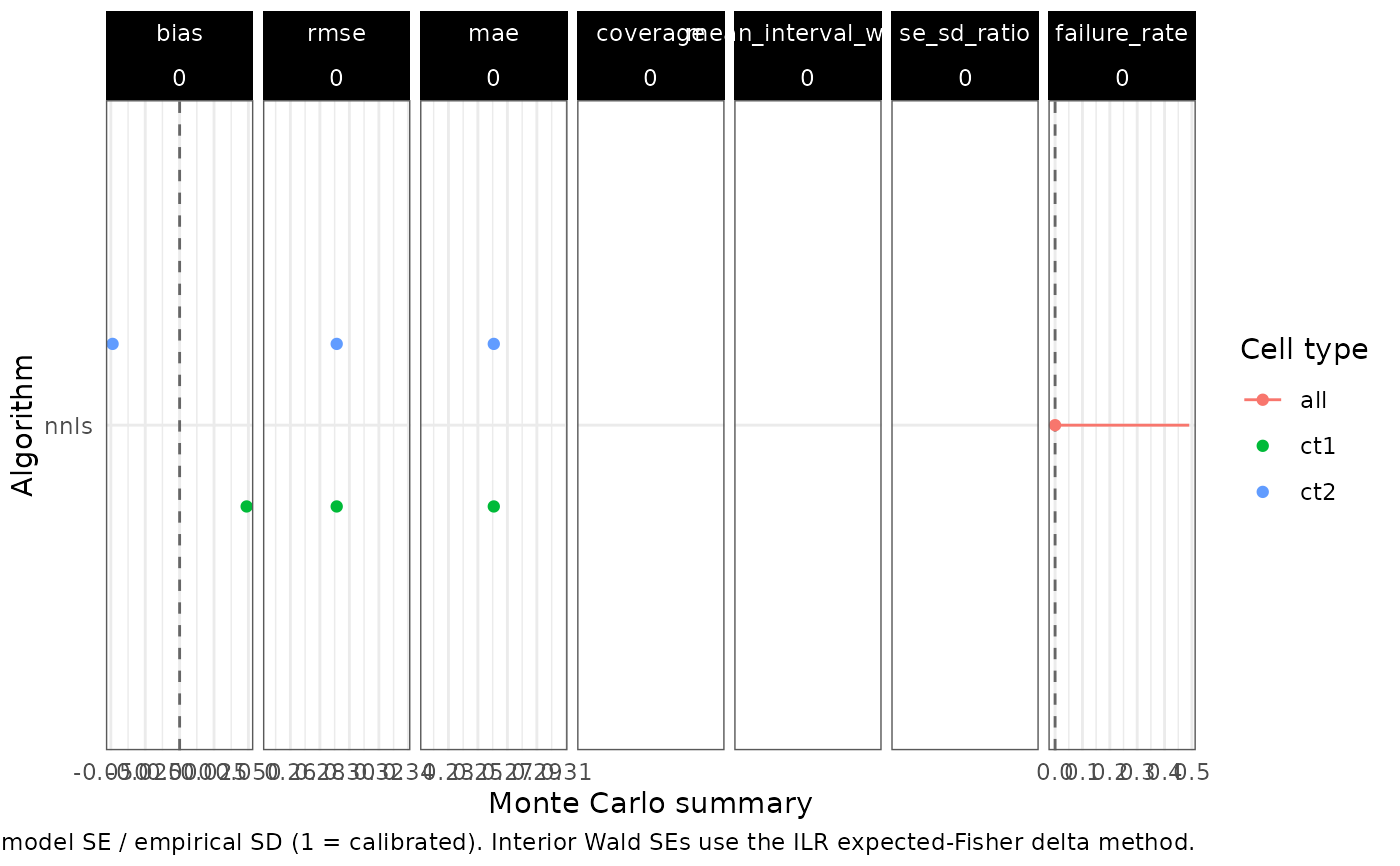
Forest plot of ADEMP Monte Carlo summaries
Source:R/04_02_benchmark_visualisation.R
plot_mc_forest.RdDot-and-whisker display of bias, RMSE, MAE, coverage, mean interval
width, SE/SD ratio, and optimiser failure rate by algorithm and cell
type
(Allen et al. 2019)
.
Coverage whiskers are the Wilson interval already stored on
monte_carlo (coverage_mc_interval();
(Wilson 1927)
): they are
intervals for the coverage rate, not for \(p_j\). Bias is
referenced at 0; coverage at 0.95; SE/SD (se_sd_ratio, mean model
SE / empirical SD) at 1. Interior Wald SEs come from
vcov_ilr_delta(). Pairwise algorithm contrasts
(MAE differences versus a reference solver on the same Monte Carlo
replicates) can be read from the raincloud of paired errors; they do
not need a second bootstrap.
Usage
plot_mc_forest(
  benchmark,
  facet_rows = NULL,
  facet_cols = NULL,
  metrics = c("bias", "rmse", "mae", "coverage", "mean_interval_width", "se_sd_ratio",
    "failure_rate")
)
Arguments
- benchmark
List from
run_simulation_benchmark(), or a table frompivot_mc_estimates().- facet_rows, facet_cols
Optional column names for
ggplot2::facet_grid()rows and columns.- metrics
Character vector of summaries to display.
References
Allen M, Poggiali D, Whitaker K, Marshall TR, van Langen J, Kievit RA (2019).
“Raincloud Plots: A Multi-Platform Tool for Robust Data Visualization.”
Wellcome Open Research, 4, 63.
ISSN 2398-502X.
doi:10.12688/wellcomeopenres.15191.2
.
https://wellcomeopenresearch.org/articles/4-63.
Wilson EB (1927).
“Probable Inference, the Law of Succession, and Statistical Inference.”
Journal of the American Statistical Association, 22(158), 209–212.
ISSN 0162-1459.
doi:10.2307/2276774
.
Examples
set.seed(1)
genes <- paste0("g", 1:2)
cts <- paste0("ct", 1:2)
mu <- matrix(c(20, 22, 22, 20), nrow = 2, dimnames = list(genes, cts))
Sigma <- array(
  c(1, 0, 0, 1, 1, 0, 0, 1),
  dim = c(2, 2, 2),
  dimnames = list(genes, genes, cts)
)
out <- run_simulation_benchmark(
  tibble::tibble(
    n_genes = 2L,
    cosine = 0,
    true_theta = list(list(p = c(0.5, 0.5), mu = mu, sigma = Sigma))
  ),
  deconvolution_functions = list(
    "nnls" = list(FUN = deconvolute_ratios_nnls)
  ),
  n = 4,
  cores = 1
)
if (requireNamespace("ggplot2", quietly = TRUE)) {
  plot_mc_forest(out, facet_cols = "cosine")
}