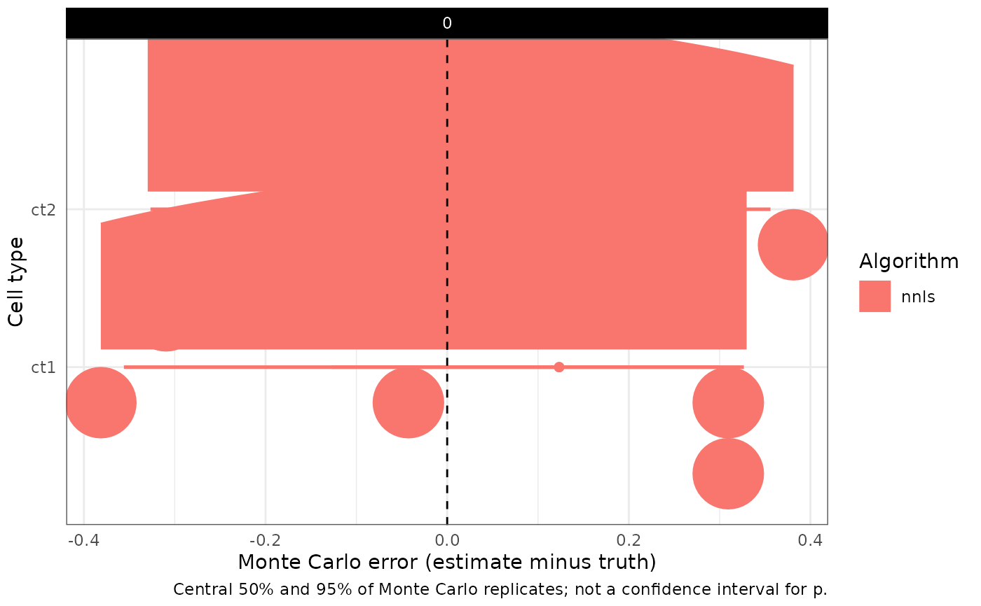
Horizontal raincloud of Monte Carlo proportion estimates

Half-eye densities, dots, and empirical 50% / 95% intervals (Allen et al. 2019) for the Monte Carlo sampling distribution of \(\hat p_j\). Default aesthetics: numeric axis is the estimation error \(\hat p_j-p_j^{\star}\) (so a vertical line at 0 is bias); the y-axis is the cell type; colour and dodge group the deconvolution algorithm. Optional facet_rows / facet_cols split scenarios (for example number of genes versus pairwise cosine).

Usage

plot_mc_raincloud(
  benchmark,
  quantity = c("error", "estimate"),
  facet_rows = NULL,
  facet_cols = NULL,
  .width = c(0.5, 0.95),
  include_dots = TRUE,
  max_dots = 2000L,
  max_rows = NULL,
  dodge_width = 0.95,
  slab_scale = 1.4,
  slab_alpha = 1,
  category_spacing = 1,
  slab = c("halfeye", "dotsinterval")
)

Arguments

benchmark: List from run_simulation_benchmark(), or a table from pivot_mc_estimates().
quantity: "error" (default) or "estimate".
facet_rows, facet_cols: Optional column names for ggplot2::facet_grid() rows and columns.
.width: Passed to ggdist::stat_halfeye(); default c(0.5, 0.95).
include_dots: If FALSE, omit ggdist::stat_dots() (use this on large Monte Carlo tables: the Fortran QP in nudge_bins cannot take long vectors).
max_dots: Maximum rows passed to stat_dots when include_dots = TRUE. Extra rows are subsampled.
max_rows: Optional cap on the plotting table (half-eye and dots). When the Monte Carlo stack is huge, subsample before drawing.
dodge_width: Width passed to ggplot2::position_dodge().
slab_scale: Slab height for ggdist::stat_halfeye().
slab_alpha: Transparency of the density slab (1 is opaque).
category_spacing: Vertical gap between discrete y categories (cell types). Values greater than 1 insert extra space so slabs from neighbouring types do not overlap; the axis still shows the original labels.
slab: "halfeye" (default KDE raincloud) or "dotsinterval" (quantile dots plus interval; avoids empty bounded slabs).

Value

A ggplot object.

Details

When quantity = "estimate" and slab = "halfeye", slabs use a bounded kernel on \([0,1]\) (ggdist::density_bounded()) with a coloured outline (slab_colour / slab_linewidth). Vertex pile-up can leave that KDE empty; slab = "dotsinterval" (ggdist::stat_dotsinterval()) draws quantile dots instead. True proportions are labelled at the top of each panel (the most abundant type to the right of its reference line; the others to the left).

The inner interval is the central 50% of Monte Carlo replicates; the outer interval is the central 95%. These are not confidence intervals for \(p_j\).

References

Allen M, Poggiali D, Whitaker K, Marshall TR, van Langen J, Kievit RA (2019). “Raincloud Plots: A Multi-Platform Tool for Robust Data Visualization.” Wellcome Open Research, 4, 63. ISSN 2398-502X. doi:10.12688/wellcomeopenres.15191.2 . https://wellcomeopenresearch.org/articles/4-63.

Examples

set.seed(1)
genes <- paste0("g", 1:2)
cts <- paste0("ct", 1:2)
mu <- matrix(c(20, 22, 22, 20), nrow = 2, dimnames = list(genes, cts))
Sigma <- array(
  c(1, 0, 0, 1, 1, 0, 0, 1),
  dim = c(2, 2, 2),
  dimnames = list(genes, genes, cts)
)
out <- run_simulation_benchmark(
  tibble::tibble(
    n_genes = 2L,
    cosine = 0,
    true_theta = list(list(p = c(0.5, 0.5), mu = mu, sigma = Sigma))
  ),
  deconvolution_functions = list(
    "nnls" = list(FUN = deconvolute_ratios_nnls)
  ),
  n = 4,
  cores = 1
)
if (requireNamespace("ggdist", quietly = TRUE)) {
  plot_mc_raincloud(out, facet_cols = "cosine")
}