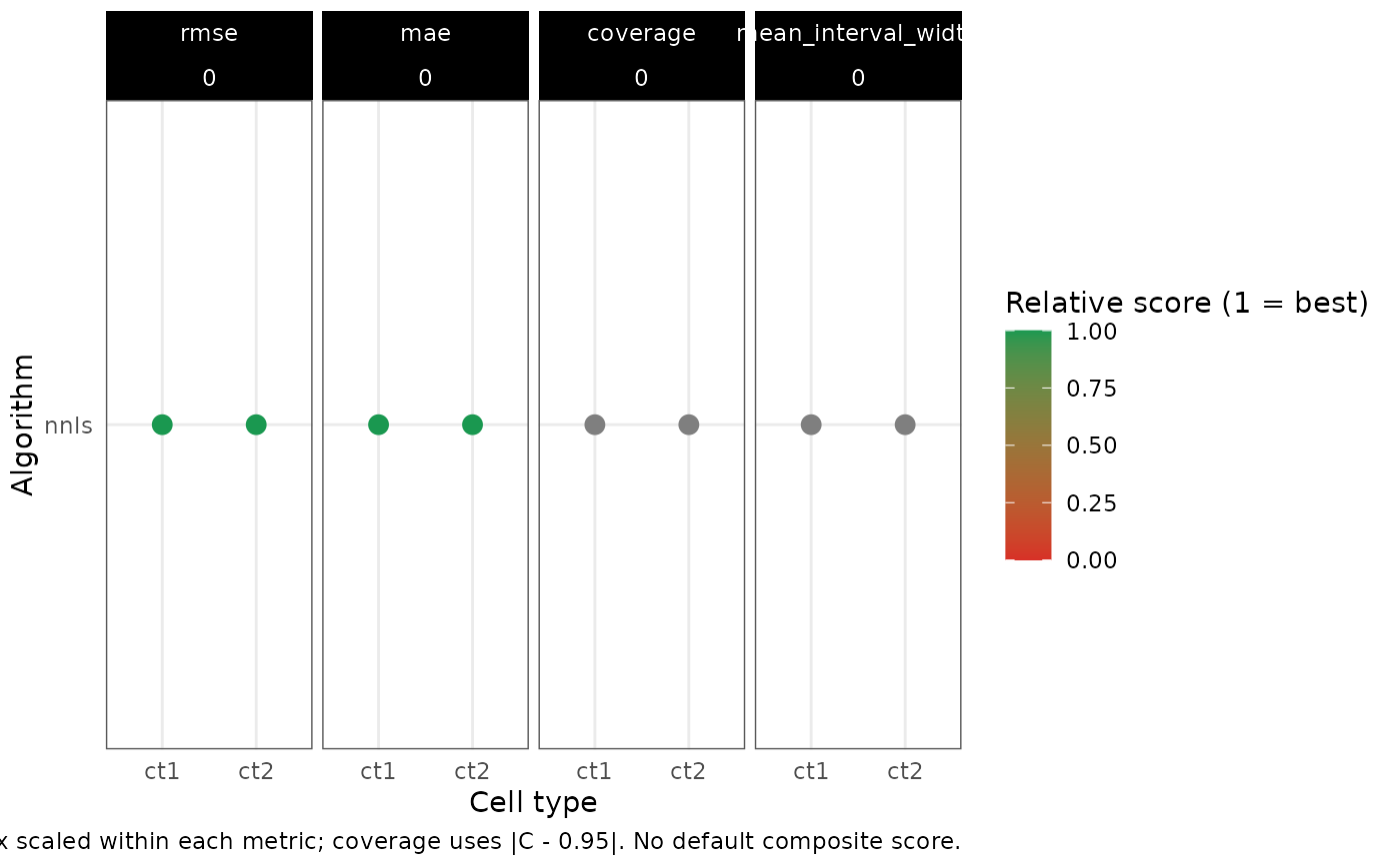
Faceted dot plot of several ADEMP metrics

One panel per metric; colour is a min-max normalised score with \(1\) = best inside that metric (and facet). Do not map a second primary score to point size. Coverage is scored as \(|\widehat C-0.95|\), so over-wide intervals that inflate coverage are not rewarded. There is no default weighted composite.

Usage

plot_mc_metric_dots(
  benchmark,
  facet_rows = NULL,
  facet_cols = NULL,
  metrics = c("rmse", "mae", "coverage", "mean_interval_width"),
  weights = NULL
)

Arguments

benchmark

List from run_simulation_benchmark(), or a table from pivot_mc_estimates().

facet_rows, facet_cols

Optional column names for ggplot2::facet_grid() rows and columns.

metrics

Character vector of summaries to display.

weights

Optional named numeric weights (sum to 1) used only to add a composite facet beside the components.

Value

A ggplot object.

See also

plot_mc_forest(), plot_algorithm_similarity()

Examples

set.seed(1)
genes <- paste0("g", 1:2)
cts <- paste0("ct", 1:2)
mu <- matrix(c(20, 22, 22, 20), nrow = 2, dimnames = list(genes, cts))
Sigma <- array(
  c(1, 0, 0, 1, 1, 0, 0, 1),
  dim = c(2, 2, 2),
  dimnames = list(genes, genes, cts)
)
out <- run_simulation_benchmark(
  tibble::tibble(
    cosine = 0,
    true_theta = list(list(p = c(0.5, 0.5), mu = mu, sigma = Sigma))
  ),
  deconvolution_functions = list(
    "nnls" = list(FUN = deconvolute_ratios_nnls)
  ),
  n = 4,
  cores = 1
)
if (requireNamespace("ggplot2", quietly = TRUE)) {
  plot_mc_metric_dots(out, facet_cols = "cosine")
}