Normalised Shannon entropy of a discrete distribution

For a probability vector \(\boldsymbol{p}\in\Delta^{J-1}\) over \(J\) classes (here: cell types), the Shannon entropy is $$ H(\boldsymbol{p}) = -\sum_{j=1}^{J} p_j \log p_j, $$ with the convention \(0\log 0 = 0\). Dividing by the maximum entropy \(\log J\) (uniform over all \(J\) classes) yields Pielou's evenness $$ H^{\star}(\boldsymbol{p}) = \frac{H(\boldsymbol{p})}{\log J} \in[0,1], $$ so \(H^{\star}=0\) for a Dirac mass on one type and \(H^{\star}=1\) for the uniform distribution over the \(J\) cell types. Zero masses are dropped only inside the sum; the normaliser still uses the original class count \(J\).

This is preferable to changing the logarithm base to the number of positive masses \(J'\), which would renormalise only on the support and hide sparsity relative to the full panel of cell types.

Usage

compute_shannon_entropy(ratios)

Arguments

ratios

Numeric vector of cellular proportions \(\boldsymbol{p}\in\Delta^{J-1}\) (length \(J\)).

Value

Scalar normalised entropy \(H^{\star}\in[0,1]\).

Illustration

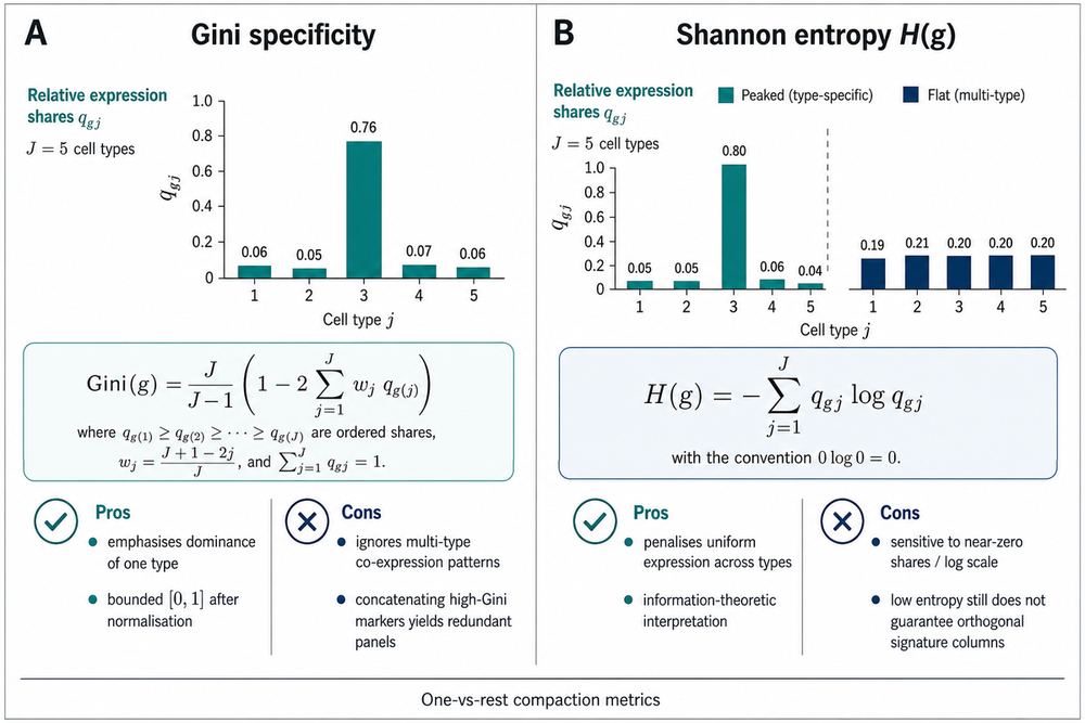
Panel B of the figure contrasts a peaked (type-specific, low entropy) share vector with a flat (multi-type, high entropy) one for \(J=5\) classes.

Examples

compute_shannon_entropy(c(1, 0, 0)) # Dirac -> 0
#> [1] 0
compute_shannon_entropy(rep(1 / 3, 3)) # uniform -> 1
#> [1] 1